Design Notes
Ross Gayler
2021-06-17
Last updated: 2021-08-18
Checks: 7 0
Knit directory:
VSA_altitude_hold/
This reproducible R Markdown analysis was created with workflowr (version 1.6.2). The Checks tab describes the reproducibility checks that were applied when the results were created. The Past versions tab lists the development history.
Great! Since the R Markdown file has been committed to the Git repository, you know the exact version of the code that produced these results.
Great job! The global environment was empty. Objects defined in the global environment can affect the analysis in your R Markdown file in unknown ways. For reproduciblity it’s best to always run the code in an empty environment.
The command set.seed(20210617) was run prior to running the code in the R Markdown file.
Setting a seed ensures that any results that rely on randomness, e.g.
subsampling or permutations, are reproducible.
Great job! Recording the operating system, R version, and package versions is critical for reproducibility.
Nice! There were no cached chunks for this analysis, so you can be confident that you successfully produced the results during this run.
Great job! Using relative paths to the files within your workflowr project makes it easier to run your code on other machines.
Great! You are using Git for version control. Tracking code development and connecting the code version to the results is critical for reproducibility.
The results in this page were generated with repository version af002d9. See the Past versions tab to see a history of the changes made to the R Markdown and HTML files.
Note that you need to be careful to ensure that all relevant files for the
analysis have been committed to Git prior to generating the results (you can
use wflow_publish or wflow_git_commit). workflowr only
checks the R Markdown file, but you know if there are other scripts or data
files that it depends on. Below is the status of the Git repository when the
results were generated:
Ignored files:
    Ignored:    .Rhistory
    Ignored:    .Rproj.user/
    Ignored:    renv/library/
    Ignored:    renv/local/
    Ignored:    renv/staging/
Note that any generated files, e.g. HTML, png, CSS, etc., are not included in this status report because it is ok for generated content to have uncommitted changes.
These are the previous versions of the repository in which changes were made
to the R Markdown (analysis/design_notes.Rmd) and HTML (docs/design_notes.html)
files. If you’ve configured a remote Git repository (see
?wflow_git_remote), click on the hyperlinks in the table below to
view the files as they were in that past version.
| File | Version | Author | Date | Message |
|---|---|---|---|---|
| Rmd | 867778a | Ross Gayler | 2021-08-11 | Add multi target simulation data |
| html | 867778a | Ross Gayler | 2021-08-11 | Add multi target simulation data |
| Rmd | 3f64430 | Ross Gayler | 2021-08-03 | Add code for VSA basic operators |
| html | 3f64430 | Ross Gayler | 2021-08-03 | Add code for VSA basic operators |
| Rmd | 7ca6f60 | Ross Gayler | 2021-07-08 | Add programming notes to design notes |
| html | 7ca6f60 | Ross Gayler | 2021-07-08 | Add programming notes to design notes |
| html | e256bf9 | Ross Gayler | 2021-07-07 | Build site. |
| Rmd | 6f799be | Ross Gayler | 2021-07-07 | Complete investigation of simulation data |
| html | 6f799be | Ross Gayler | 2021-07-07 | Complete investigation of simulation data |
| Rmd | a683bb1 | Ross Gayler | 2021-07-07 | Complete investigation of simulation data |
| html | a683bb1 | Ross Gayler | 2021-07-07 | Complete investigation of simulation data |
| html | 7eae4c3 | Ross Gayler | 2021-06-26 | Check simulation data: initial values and z versus dz |
| Rmd | c39cb39 | Ross Gayler | 2021-06-25 | Take first look at simulation data |
| html | c39cb39 | Ross Gayler | 2021-06-25 | Take first look at simulation data |
| Rmd | 456a363 | Ross Gayler | 2021-06-21 | Add automatic rendering of DFDs |
| html | 456a363 | Ross Gayler | 2021-06-21 | Add automatic rendering of DFDs |
| Rmd | d8b9d53 | Ross Gayler | 2021-06-18 | Add DFD for Design 01 |
| html | d8b9d53 | Ross Gayler | 2021-06-18 | Add DFD for Design 01 |
| Rmd | 0b7e1d4 | Ross Gayler | 2021-06-17 | Publish initial docs |
| html | 0b7e1d4 | Ross Gayler | 2021-06-17 | Publish initial docs |
This notebook records the design considerations behind implementing altitude hold in VSA.
1 Drop-in strategy
Limit the initial problem to altitude hold because this is one-dimensional (as opposed to fully general flight control). This is done to simplify the problem as much as possible.
Treat the VSA components as drop-in replacements for standard control circuitry. This reduces the probability that we will hit an obstacle requiring us to completely reconceptualise how altitude hold is done. On the other hand, it means that we will parallel the classical altitude hold computation, so we may miss seeing some (hypothetical) VSA-centric solution that has no classical analogue.
Drop-in replacement, taken literally, implies replacement of individual functions (single nodes) of the data flow diagram. These are generally simple functions, so could reasonably be designed (rather than learned). However, it is also possible to replace larger subsets of the data flow diagram. As these subsets get larger the function computed becomes more complex and design becomes less attractive relative to learning.
The initial intent is to build the system by design, which implies one for one replacement of the PID components with VSA equivalents. If there is time (or necessity) we will try to learn the replacement VSA components and move from one for one replacement to a holistic re-implementation of the PID controller.
1.1 Idealisation versus implementation
A drop-in replacement strategy is not necessarily as straight-forward as it sounds. This is primarily due to the unnoticed heavy lifting that is done by the idealised mathematical abstractions we habitually use.
1.1.1 Range and resolution
The values manipulated by the PID controller are modelled mathematically as real numbers, which are unbounded and have arbitrarily fine resolution (infinite precision). However, any physical implementation will have limited range and resolution.
An implementation on a digital computer would probably represent the real scalars with floating point numbers. These have a sufficiently wide range and sufficiently fine resolution that the limitations relative to real numbers can generally be ignored. However, as the representational and computational resources are reduced the probability that the limitations will have visible effects on the behaviour of the PID controller increases.
One of the purposes of using a VSA approach in robotics is to attempt to achieve computation with fewer resources, which may mean we are operating in the regime where representational limits are relevant. While it is possible we may never approach those limits in this work it is appropriate to always keep in mind that those limits do exist for VSAs. In particular, we will treat all scalar values as being bounded.
1.1.2 Scaling
In a mathematical model the quantities are unscaled, they are just numbers (e.g. Langtangen & Pedersen (2016) first paragraph of the preface). However, in an implementation the numbers (especially coming from sensors) are necessarily scaled. (Is the vertical velocity measured in metres per second or furlongs per fortnight?) Quantities to be combined by some function need to be scaled compatibly. For example, if we are adding two vertical velocities they should be identically scaled for standard addition to have the desired effect.
In a VSA system we are close to the mathematical idealisation, in that the VSA representation of a magnitude carries no indication of the scaling. If we had a VSA implementation of the standard addition operator we would need to ensure that the representations of the arguments were compatibly scaled. However, if we are effectively learning an addition operator to be used in a specific context there is no need for the arguments to be compatibly scaled because we learn the appropriate scaling of the arguments as part of learning the addition operator.
Consider an extended example by looking at the PID calculation of error
(\(e\)): \[
\begin{aligned}
e &= k_{tgt} - z - dz \\
&= k_{tgt} - (z + dz)
\end{aligned}
\]
The term \((z + dz)\) is effectively a prediction of the altitude at some time in the future. The altitude \(z\) happens to be supplied scaled as metres and the vertical velocity happens to be supplied scaled in metres per second. In order for \(z\) and \(dz\) to be scaled compatibly, so they can be combined with the standard addition operator we can take the implied prediction interval to be one second, so that \(dz\) is interpreted as the distance in metres that will be covered in the next second. (The mathematical notation is arguably misleading and should contain an explicit multiplication of the vertical velocity by the prediction period, however that just illustrates that the mathematical idealisation makes it possible to ignore implementation details.)
So, \(e\) can be interpreted as the predicted altitude error in one second assuming no change in vertical velocity. However, the whole point of the PID controller is to vary the vertical velocity of the multicopter, eventually bring it to zero. In addition, the response rate of the system is sufficiently high (100 time steps per second) that the vertical velocity of the multicopter is likely to vary significantly over the one second prediction interval, thus invalidating the prediction.
Consequently, the one second prediction horizon implied by the scaling of the inputs is likely to be rather longer than appropriate for optimal control. Presumably this gets compensated for by the tuning parameters of the PID controller. So if the VSA version is designed (rather than learned) it will be limited by the quality of the tuning of the controller. On the other hand if the VSA functions are learned, there is an opportunity for the optimal scaling to be learned to best match the response rate of the system.
1.1.3 Propagation delays
Treating the PID controller as a mathematical idealisation it is simplest to assume that values propagate instantaneously through the DFD. This means that the functional input/output relations of the nodes can be treated as equations. A physical implementation would necessarily have propagation delays. In a neuromorphic implementation the propagation delays are probably essential to the dynamics of the system.
2 Design issues
2.1 VSA implementation
There is much more to follow on the VSA implementation. I will expand this later, but wanted to publish the VSA implementation code first.
Most of the points raised in this section will be directly relevant to the design choices in implementing the VSA operations for this project. However, some points may be more general observations that are not immediately relevant to this project.
2.1.1 VSA type
There are multiple possible VSA implementations, e.g. see als@schlegelComparisonVectorSymbolic2020 and Kleyko et al. (2021) . I need to choose an appropriate implementation.
Every vector has a magnitude (a single degree of freedom scalar value) and a direction (a many degree of freedom value)
- Construing the vector in terms of magnitude and direction rather than in terms of the basis elements is a choice made by the analyst for task-relevant reasons. The best reasons are where that decomposition relates directly to the functional roles of those components in the operation of the system.
- I am using the ‘analog computer’ interpretation of VSA systems. The direction of the vector is a systematically constructed label indicating what the vector represents (corresponds to). The magnitude of the vector indicates the degree of support for the represented thing in the VSA computation. (Thinking of this as an electronic analog computer, the vector direction corresponds to a wire and the vector magnitude corresponds to the voltage on the wire (gayler2013?).)
- In that ‘analog computer’ interpretation the vector magnitude is relevant only to the dynamics of the VSA system and not to the representations. That is, the vector magnitude is a computational resource and not a representational resource. So, only the directions of the VSA vectors are representationally relevant.
In this project all the quantities of interest are scalars, so modelling functions of scalars is central to the project. Given that we will end up using a regression-like approach to learn functions between scalars I am concerned that the regression might exploit vector magnitudes (rather than vector directions). Consequently, I want to choose a VSA type that reduces the opportunity for regression to depend on the magnitude rather than
Use the MAP-B type ((Schlegel, Neubert, & Protzel, 2020, Table 1; Gayler, 1998)). This is also referred to as bipolar VSA. Each VSA vector \(X \in \{-1, 1\}^D\).
2.1.2 VSA similarity
- VSA representations are thoroughly distributed, in the sense that, as much as possible, the underlying basis elements should be irrelevant to the operation of the system.
2.2 PID controller
The existing classically implemented computation is a PID controller
By my reading there is no claim to the optimality of PID controllers. Rather, they are simple, do not require a model of the controlled system, and are in widespread use.
My reading also suggests there are plenty of PID variants that are pragmatic engineering solutions to issues with the idealised basic PID.
I conclude there is nothing sacrosanct about PID control, and it is possible that other PID variants or completely different approaches to process control may be more amenable to VSA implementation.
Nonetheless, I will stick with attempting a VSA implementation of the existing PID controller because of the commitment to a drop-in replacement strategy.
The concept of drop-in replacement makes most sense when replacing individual components of the data flow graph.
VSA replacement of larger components of the data flow graph (in the extreme, treating the entire PID controller as a single VSA function) arguably loses the PID structure, because those components no longer exist as separable mechanisms.
2.3 Parameterisation
The classically implemented PID controller has four parameters: \(k_{tgt}\), \(k_p\), \(k_i\), \(k_{windup}\)
\(k_{tgt}\), the target holding altitude, should arguably be a variable rather than a parameter. In the current implementation it is set to the constant value of 5 metres. A more general implementation would allow the hold altitude to be set arbitrarily.
- If this is treated as a variable it will need to be explicitly represented as a VSA value even if the value is held constant during simulations.
- Parameters which are treated as constants do not need to be explicitly represented as VSA values and their effect can be absorbed into the surrounding function (like currying)
The remaining three parameters are for tuning the PID process to minimise overshoot and other undesired behaviours.
There are interactions between the parameters (in terms of their joint effect on the system behaviour).
- For example, \(k_i\) is relatively large in the classically implemented system at least in part to compensate for \(k_{windup}\) being relatively small.
VSA representations of scalar values have a limited range, which must be specified.
Consequently, I have guessed what might be plausible ranges for the parameters if they were to be treated as variables. Don’t takes these ranges too seriously.
The values of some variables in the data flow graph are functions of the parameters, so the ranges of these variables depend in part on the ranges I have guessed for the parameters.
The specific parameterisation of the classically implemented PID controller may not be the most amenable to VSA implementation. For example, the wide value range for some variables caused by the (guessed) wide value range for some parameters may have the effect of making the computation more noisy.
- The parameters \(k_p\) and \(k_i\) effectively control the relativel contribution of the error and integrated error terms to the motor demand. If the error and integrated error variables were scaled to have identical ranges and \(k_p\) scaled to the range \([0, 1]\) then the two terms could be weighted by \(k_p\) and \(1 - k_p\) respectively, which would probably be better for VSA implementation.
2.4 Interfacing
How do we interface between the VSA components and the classical components?
VSA values are very high dimensional vectors.
The values in the classical implementation of the data flow diagram are very low dimensional vectors (typically scalars).
The surrounding machinery of the multicopter simulation assumes that the inputs to and outputs from the altitude hold are classical values. Therefore interfaces are need to convert between the classical and VSA representations.
The interfaces between the classical and VSA are essentially projections between low and high dimensional vector spaces.
2.5 Representation of scalars
- Magnitude vs. spatial
2.5.1 Range limits
2.5.2 Value resolution and noise
VSA representations, like any physical implementation have limited value resolution (i.e. two scalar values which are sufficiently close will be indistinguishable).
Value resolution hasn’t been investigated in the VSA literature, but it is clear that it won’t be a sharp distinction (e.g. as in binary representations). Rather, it is more likely to be a probabilistic effect - the closer the two values, the higher the probability that their two VSA representations are indistinguishable. If this is the case, then the value resolution can be thought of as equivalent to adding random noise to the value, making the “true” value unobservable and uncertain.
I expect VSA resolution to be increased by increasing the dimensionality of the vector space.
I also expect VSA resolution to be increased by using the ensemble averaging technique used in the multiset intersection circuit (Gayler & Levy, 2009).
I expect that the initial VSA designs will be thoroughly over-resourced, so that they have far finer value resolution than is necessary for implementation of the PID controller.
2.6 Temporal issues
Standard VSA is point-in-time/static (some implementations may be inherently temporal)
Embedded in discrete-time simulation. Compatibility of time scales.
Temporal resolution of signals?
Low-pass filters on everything?
2.7 Initialisation
- Classical implementation has explicit initialisation. Do we need special VSA circuits to guarantee orderly turn-on? Could we have an “always-on” VSA design?
2.8 Simulation program
These are issues that relate to the simulations as software artefacts.
2.8.1 Relation of VSA and multicopter simulation components
Ross Gayler will program the initial VSA work in R because he is a tolerable R programmer and useless in Python.
Simon Levy has programmed the multicopter simulation in Python. Simon is an excellent programmer in multiple languages, but not experienced in R.
At some point the VSA controller code will need to be implemented in the multicopter simulation. The current plan is that the VSA computation would be reimplemented from R to Python.
- It is possible to interoperate R and Python, but adding extra dependencies to the gym-copter project is unattractive, and the R implementation of the VSA operations will have features (e.g. retention of all history) that are not appropriate in a more operational environment.
The current plan is that the R VSA implementation of the altitude hold controller will only implement the controller, and not the multicopter simulation it is embedded in.
The VSA altitude controller will be “trained” using files of input and output values generated by the multicopter simulation. This will be offline, so there will be no opportunity for unexpected outputs from the altitude controller to be fed back into the multicopter simulation.
- If online training becomes necessary the VSA component will have to be embedded in the multicopter simulation or some way of coupling the two systems developed.
2.8.2 Structure of the VSA data flow graph implementation
Some initial exploratory VSA work can be done as standalone analyses (e.g. exploration of value encoding schemes). However, any implementation of the data flow graph will require a more systematic approach, as follows:
The history of the state of the system will be represented by a data frame (actually, a tibble, because I will need to use list columns to hold the VSA representations).
- The history of the state is required so that we can plot the state trajectory and diagnose problems with the dynamics.
Each row of the data frame corresponds to a discrete time step, \(t = 1:n\) (\(n\) will be fixed for any run of the system).
- There will be an extra initial time step (\(t = 0\)) corresponding to the initial values of the state variables.
Each column of the data frame corresponds to an input variable, an internal state variable of the altitude controller, an output variable, or the time variable (\(t\)).
- The input and output variables are numeric scalars. The internal state variables are scalars in the classical implementation, but will be high-dimensional vectors in the VSA implementation.
The values of the input and (desired) output variables are known in advance for every time.
The values of the internal state variables are initially only known for the start time, \(t = 0\).
At each time step \(t\) a state update function is applied to the \(t\) row of the state history to calculate the next row of the state-history (\(time = t + 1\)).
The state and output variables are a function of the current input variables and the previous state variables.
For efficiency reasons, the accumulation of rows into a data frame is implemented by generating each row as a one-row data frame, accumulating those one-row data frames as elements of a list, then bulk-converting the list of one-row data frames to a single data frame (see https://win-vector.com/2015/07/27/efficient-accumulation-in-r/ & https://dplyr.tidyverse.org/reference/rows.html)
2.8.3 Timing skew
There is potential issue to be watched out for concerning the relative timing of the input, state, and output variables in the state-history data frame.
Each row of the state-history data frame corresponds to a unique time \(t\). Each column of the data frame corresponds to a variable. So the values of the variables in the same row should all represent measurements made at the same time \(t\).
The variables in the state-history data frame correspond to nodes in the data flow graph. The requirement for all variables in a row to be measured at the same time is equivalent to saying that values propagate instantaneously through the data flow graph.
Because we know that in reality there are propagation delays we are tempted to assume that the inputs precede the outputs. This could translate into effectively making the output at \(t\) a function of the inputs at \(t - 1\). We need to be vigilant to ensure this does not happen. (This might be hard to spot in the multicopter simulation code because the variables are not explicitly time subscripted and the state component updates are probably applied progressively throughout the code rather being applied in a single atomic update.)
3 Design 01 - No VSA
This section deals with the altitude hold controller before the introduction of any VSA components.
3.1 Data Flow Diagram
The data flow diagram represents the desired calculation for altitude hold.
The data flow diagram is derived from
AltitudeHoldPidController.Each node in the diagram represents a potentially inspectable value or the application of a function
Each directed edge in the diagram represents a value flow from one node to another
Think of the data flow diagram as specifying an electronic analog computer where the nodes correspond to function blocks and the edges correspond to wires.
This is the diagram supplied by Simon Levy.
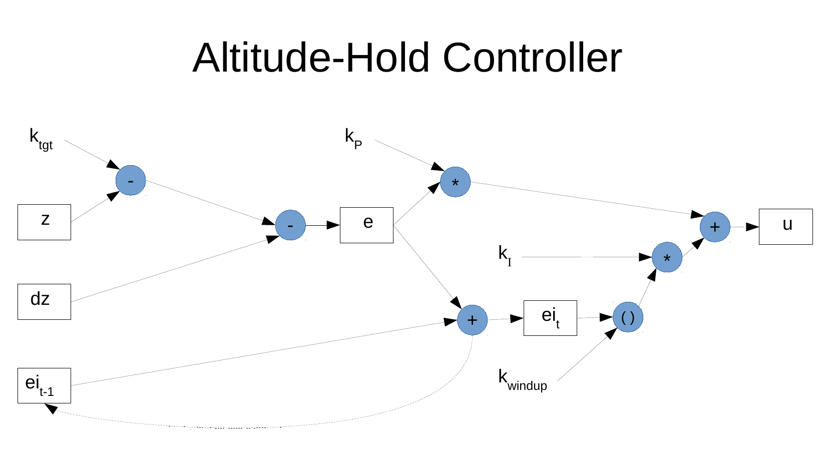
Each node should be interpreted as being implicitly subscripted by time. Only the ei nodes are explicitly subscripted by time.
The value of the u node is constrained to the range [0, 1]. This can be interpreted as implying that there should be an application of a function to constrain the value to that range. This will be inserted in the diagram below.
The integrated error \(ei_t\) is actually implemented as the integration after the clipping by \(k_{windup}\) is applied. (This is corrected in the following diagram.)
The following diagram has been reformatted to be consistent with later data flow diagrams.
Parameter nodes are coloured white. These are constant values.
Input nodes are coloured light yellow. These are variable values over time.
Output nodes are coloured dark yellow These are variable values over time.
Internal nodes are coloured cyan. These are variable values over time.
All the internal nodes and the output node implement functions with variable values over time.
All functions except subtraction are commutative, so the mapping from input edges to function arguments is irrelevant.
Because the subtraction function is non-commutative, the two input edges must be mapped to the correct function arguments. The edges are labelled “+” (first argument) and “-” (second argument).
This data flow diagram represents the classically implemented computation, so each value is a scalar real.
Each node is labelled so that they can be referred to.
- The function nodes are labelled with the function name, then a unique label in parentheses.
Each node should be interpreted as being a value implicitly subscripted by time.
The magenta coloured nodes represent reference values. These are imported from the classically implemented simulations which are equivalent to a corresponding node in the data flow diagram. The values of the reference node and the corresponding node should be identical (up to approximation error).
The edge between a reference node and the corresponding node is labelled “=” to indicate that it is only intended for testing the calculation and is not actually part of the data flow diagram.
The calculation (and hence, interpretation) of the \(u\) node varies between simulation data files.
- In some files (\(u_{clip} = TRUE\)) the value was exported after clipping, so should be identical to the value of node \(i8\).
- In the remaining files (\(u_{clip} = FALSE\)) the value was exported before clipping, so should be identical to the value of node \(i7\).
3.2 Data flow tables
The data flow diagram is specified in an external spreadsheet. This allows extra attributes to be associated with the nodes and edges and provides a tolerable user interface for editing the specifications. These tables record more detail about the data flow diagram than can be reasonably displayed on the data flow graph.
For each value (node) , what is it’s range? A physical implementation necessarily has limits. This may render \(k_{windup}\) and
constrainredundant.I have guessed values for the ranges of the variables (informed by the analysis of the simulation data).
The ranges for the parameters are truly plucked from the air.
For each value (node) , what is it’s value resolution? This is equivalent asking the noise level that can be tolerated.
For each value (node) , what is it’s temporal resolution? This is equivalent how rapidly we expect the value to change. Some nodes are constant parameters. For time-varying signals do we expect them to alternate between the extreme values on successive samples?
A related point: this is a discrete-time simulation - is the time step fixed? What is the time step? The simplest VSA approach is point-in-time. However, it may be possible to dream up some VSA representation that is essentially temporal, in which case it needs to be compatible with the time-scales of the implementation.
Are there better descriptions for the internal nodes? Something with intuitive meaning of their function would be good.
Does the integrated error needs to be initialised to zero? Does this imply the need for “turn-on” circuitry? Would it be better to have an “always-on” design? Should there be some error correction for cumulative errors?
4 Design 02 - No VSA (tidied)
This is the previous design modified to be more compatible with the VSA changes which will be introduced later.
5 Extreme designs
Digress briefly to consider the extremes of where we might go with incorporating VSA components into the design of the altitude hold circuit.
5.1 Minimal collapse
Replace all the edges in the data flow diagram with VSA equivalents.
Leave all the vertices in classical form.
The edges are equivalent to wires. A value is inserted at one end and retrieved at the other end. This would require a classical to VSA interface at the input of the edge and a VSA to classical interface at the output end.
This would seem to be an almost pointless thing to do. However, the classical values are assumed to absolutely accurate as mathematical idealisations. Different physical realisations will be inaccurate to some extent. A software implementation would likely represent the values as double-precision floating-point. A very constrained computer might represent the values with 8-bit integers. An analog computer might represent the values as voltages in some constrained range and with noise present in the signal.
Analogously, there can be range, distortion, and noise effects present in VSA representations. There can also be implementation noise, for example if VSA representations are implemented with simulated spiking neurons.
- The minimal collapse scenario would be useful for investigating the effects of VSA representation inaccuracy on the behaviour of the otherwise unaltered altitude hold circuit. This could indicate which values require high fidelity representations.
5.2 Maximal collapse
- Replace the entire set of vertices of the data flow diagram (with the exception of external sources and sinks) with a single vertex. That is, altitude hold is treated as a single, complicated function with no discernible internal data flows. For example, it might be possible to implement the altitude hold as effectively an interpolating lookup table.
Such a model might have advantages depending on the implementation technology.
6 Design 03 -
7 Design 04 -
8 Etc.
References
R version 4.1.1 (2021-08-10)
Platform: x86_64-pc-linux-gnu (64-bit)
Running under: Ubuntu 21.04

Matrix products: default
BLAS:   /usr/lib/x86_64-linux-gnu/blas/libblas.so.3.9.0
LAPACK: /usr/lib/x86_64-linux-gnu/lapack/liblapack.so.3.9.0

locale:
 [1] LC_CTYPE=en_AU.UTF-8       LC_NUMERIC=C
 [3] LC_TIME=en_AU.UTF-8        LC_COLLATE=en_AU.UTF-8
 [5] LC_MONETARY=en_AU.UTF-8    LC_MESSAGES=en_AU.UTF-8
 [7] LC_PAPER=en_AU.UTF-8       LC_NAME=C
 [9] LC_ADDRESS=C               LC_TELEPHONE=C
[11] LC_MEASUREMENT=en_AU.UTF-8 LC_IDENTIFICATION=C

attached base packages:
[1] stats     graphics  grDevices datasets  utils     methods   base

other attached packages:
[1] tibble_3.1.3       Matrix_1.3-4       purrr_0.3.4        DT_0.18
[5] dplyr_1.0.7        DiagrammeR_1.0.6.1 readxl_1.3.1       here_1.0.1

loaded via a namespace (and not attached):
 [1] Rcpp_1.0.7         pillar_1.6.2       compiler_4.1.1     cellranger_1.1.0
 [5] later_1.2.0        RColorBrewer_1.1-2 git2r_0.28.0       workflowr_1.6.2
 [9] tools_4.1.1        digest_0.6.27      lattice_0.20-44    jsonlite_1.7.2
[13] evaluate_0.14      lifecycle_1.0.0    pkgconfig_2.0.3    rlang_0.4.11
[17] rstudioapi_0.13    crosstalk_1.1.1    yaml_2.2.1         xfun_0.25
[21] stringr_1.4.0      knitr_1.33         generics_0.1.0     fs_1.5.0
[25] vctrs_0.3.8        htmlwidgets_1.5.3  grid_4.1.1         tidyselect_1.1.1
[29] rprojroot_2.0.2    glue_1.4.2         R6_2.5.0           fansi_0.5.0
[33] rmarkdown_2.10     bookdown_0.22      tidyr_1.1.3        magrittr_2.0.1
[37] whisker_0.4        promises_1.2.0.1   ellipsis_0.3.2     htmltools_0.5.1.1
[41] renv_0.14.0        httpuv_1.6.1       utf8_1.2.2         stringi_1.7.3
[45] visNetwork_2.0.9   crayon_1.4.1