[meta] Check residenial variables
m_01_6_check_resid
Ross Gayler
2021-05-15
Last updated: 2021-05-27
Checks: 7 0
Knit directory:
fa_sim_cal/
This reproducible R Markdown analysis was created with workflowr (version 1.6.2). The Checks tab describes the reproducibility checks that were applied when the results were created. The Past versions tab lists the development history.
Great! Since the R Markdown file has been committed to the Git repository, you know the exact version of the code that produced these results.
Great job! The global environment was empty. Objects defined in the global environment can affect the analysis in your R Markdown file in unknown ways. For reproduciblity it’s best to always run the code in an empty environment.
The command set.seed(20201104) was run prior to running the code in the R Markdown file.
Setting a seed ensures that any results that rely on randomness, e.g.
subsampling or permutations, are reproducible.
Great job! Recording the operating system, R version, and package versions is critical for reproducibility.
Nice! There were no cached chunks for this analysis, so you can be confident that you successfully produced the results during this run.
Great job! Using relative paths to the files within your workflowr project makes it easier to run your code on other machines.
Great! You are using Git for version control. Tracking code development and connecting the code version to the results is critical for reproducibility.
The results in this page were generated with repository version a6fb2e3. See the Past versions tab to see a history of the changes made to the R Markdown and HTML files.
Note that you need to be careful to ensure that all relevant files for the
analysis have been committed to Git prior to generating the results (you can
use wflow_publish or wflow_git_commit). workflowr only
checks the R Markdown file, but you know if there are other scripts or data
files that it depends on. Below is the status of the Git repository when the
results were generated:
Ignored files:
    Ignored:    .Rhistory
    Ignored:    .Rproj.user/
    Ignored:    .tresorit/
    Ignored:    _targets/
    Ignored:    data/VR_20051125.txt.xz
    Ignored:    data/VR_Snapshot_20081104.txt.xz
    Ignored:    renv/library/
    Ignored:    renv/local/
    Ignored:    renv/staging/

Unstaged changes:
    Modified:   analysis/m_00_status.Rmd
Note that any generated files, e.g. HTML, png, CSS, etc., are not included in this status report because it is ok for generated content to have uncommitted changes.
These are the previous versions of the repository in which changes were made
to the R Markdown (analysis/m_01_6_check_resid.Rmd) and HTML (docs/m_01_6_check_resid.html)
files. If you’ve configured a remote Git repository (see
?wflow_git_remote), click on the hyperlinks in the table below to
view the files as they were in that past version.
| File | Version | Author | Date | Message |
|---|---|---|---|---|
| Rmd | ab90fe6 | Ross Gayler | 2021-05-18 | WIP |
| html | ab90fe6 | Ross Gayler | 2021-05-18 | WIP |
| Rmd | 1499235 | Ross Gayler | 2021-05-16 | WIP |
| Rmd | 24d95c0 | Ross Gayler | 2021-05-15 | WIP |
| Rmd | 411de1e | Ross Gayler | 2021-04-04 | WIP |
| html | 411de1e | Ross Gayler | 2021-04-04 | WIP |
| Rmd | 0bd4a5f | Ross Gayler | 2021-04-03 | WIP |
| html | 0bd4a5f | Ross Gayler | 2021-04-03 | WIP |
| Rmd | 9b4272d | Ross Gayler | 2021-04-02 | WIP |
| html | 9b4272d | Ross Gayler | 2021-04-02 | WIP |
# NOTE this notebook can be run manually or automatically by {targets}
# So load the packages required by this notebook here
# rather than relying on _targets.R to load them.

# Set up the project environment, because {workflowr} knits each Rmd file
# in a new R session, and doesn't execute the project .Rprofile

library(targets) # access data from the targets cache

library(tictoc) # capture execution time
library(here) # construct file paths relative to project root
here() starts at /home/ross/RG/projects/academic/entity_resolution/fa_sim_cal_TOP/fa_sim_callibrary(fs) # file system operations
library(dplyr) # data wrangling
Attaching package: 'dplyr'The following objects are masked from 'package:stats':
filter, lagThe following objects are masked from 'package:base':
intersect, setdiff, setequal, unionlibrary(gt) # table formatting
library(stringr) # string matching
library(vroom) # fast reading of delimited text files
library(lubridate) # date parsing
Attaching package: 'lubridate'The following objects are masked from 'package:base':
date, intersect, setdiff, unionlibrary(forcats) # manipulation of factors
library(ggplot2) # graphics
library(skimr) # compact summary of each variable
library(tidyr) # data tidying
# start the execution time clock
tictoc::tic("Computation time (excl. render)")
# Get the path to the raw entity data file
# This is a target managed by {targets}
f_entity_raw_tsv <- tar_read(c_raw_entity_data_file)1 Introduction
These meta notebooks document the development of functions that will be applied in the core pipeline.
The aim of the m_01 set of meta notebooks is to work out how to read the
raw entity data, drop excluded cases, discard irrelevant variables,
apply any cleaning, and construct standardised names. This does not
include construction of any modelling features. To be clear, the target
(c_raw_entity_data) corresponding to the objective of this set of
notebooks is the cleaned and standardised raw data, before constructing
any modelling features.
This notebook documents the checking of the “residential” variables for any issues that need fixing. These are the residential address and the phone number (which is tied to the address if the telephone is a land-line).
The subsequent notebooks in this set will develop the other functions needed to generate the cleaned and standardised data.
Regardless of whether there are any issues that need to be fixed, the analyses here may inform our use of these variables in later analyses.
We have no intention of using the residence variables as predictors for entity resolution. However, they may be of use for manually checking the results of entity resolution. Consequently, the checking done here is minimal.
Define the residential variables:
unit_num- Residential address unit numberhouse_num- Residential address street numberhalf_code- Residential address street number half codestreet_dir- Residential address street direction (N,S,E,W,NE,SW, etc.)street_name- Residential address street namestreet_type_cd- Residential address street type (RD, ST, DR, BLVD, etc.)street_sufx_cd- Residential address street suffix (BUS, EXT, and directional)res_city_desc- Residential address city namestate_cd- Residential address state codezip_code- Residential address zip codearea_cd- Area code for phone numberphone_num- Telephone number
vars_resid <- c(
  "unit_num", "house_num",
  "half_code", "street_dir", "street_name", "street_type_cd", "street_sufx_cd",
  "res_city_desc", "state_cd", "zip_code",
  "area_cd", "phone_num"
)
2 Read entity data
Read the raw entity data file using the previously defined core pipeline
functions raw_entity_data_read(), raw_entity_data_excl_status(),
raw_entity_data_excl_test(), raw_entity_data_drop_novar(),
raw_entity_data_parse_dates(), and raw_entity_data_drop_cancel_dt().
# Show the data file name
fs::path_file(f_entity_raw_tsv)
[1] "VR_20051125.txt.xz"d <- raw_entity_data_read(f_entity_raw_tsv) %>%
raw_entity_data_excl_status() %>%
raw_entity_data_excl_test() %>%
raw_entity_data_drop_novar() %>%
raw_entity_data_parse_dates() %>%
raw_entity_data_drop_admin()
dim(d)[1] 4099699 223 Dwelling
unit_num- Residential address unit numberhouse_num- Residential address street numberhalf_code- Residential address street number half code
d %>%
  dplyr::select(unit_num, house_num, half_code) %>%
skimr::skim()| Name | Piped data |
| Number of rows | 4099699 |
| Number of columns | 3 |
| _______________________ | |
| Column type frequency: | |
| character | 3 |
| ________________________ | |
| Group variables | None |
Variable type: character
| skim_variable | n_missing | complete_rate | min | max | empty | n_unique | whitespace |
|---|---|---|---|---|---|---|---|
| unit_num | 3755239 | 0.08 | 1 | 7 | 0 | 16116 | 0 |
| house_num | 0 | 1.00 | 1 | 6 | 0 | 27534 | 0 |
| half_code | 4088996 | 0.00 | 1 | 1 | 0 | 41 | 0 |
We are mostly interested in how much these fields are used, so
concentrate on complete_rate.
All these variables are character variables, so min and max refer to
the minimum and maximum lengths of the values as character strings.
The number of unique values, n_unique, is also of interest.
unit_num- 8% filled
- There are some awfully long unit numbers
- There are an awful lot of unique unit numbers
house_num- 100% filled
- There are some awfully long house numbers
- There are an awful lot of unique house numbers
half_code0.3% filled- All exactly 1 character long
- There are more unique values than I would expect for a one character string
3.1 unit_num
unit_num- Residential address unit number
Look at some examples grouped by length
d %>%
  dplyr::select(unit_num) %>%
  dplyr::filter(!is.na(unit_num)) %>%
  dplyr::mutate(length = stringr::str_length(unit_num)) %>%
  dplyr::group_by(length) %>%
  dplyr::count(unit_num) %>% # count occurrences of each unique value
  dplyr::slice_max(order_by = n, n = 5) %>%
  gt::gt() %>%
  gt::opt_row_striping() %>%
  gt::tab_style(style = cell_text(weight = "bold"), locations = cells_column_labels()) %>%
  gt::fmt_missing(columns = everything(), missing_text = "<NA>") %>%
gt::fmt_number(columns = n, decimals = 0)| unit_num | n |
|---|---|
| 1 | |
| A | 28,214 |
| B | 26,535 |
| C | 14,240 |
| D | 12,452 |
| E | 7,956 |
| 2 | |
| 10 | 2,090 |
| 11 | 1,878 |
| 12 | 1,844 |
| 14 | 1,390 |
| 13 | 1,378 |
| 3 | |
| 102 | 2,579 |
| 101 | 2,499 |
| 103 | 2,296 |
| 201 | 2,205 |
| 104 | 2,201 |
| 4 | |
| APTB | 194 |
| APTA | 185 |
| APTC | 106 |
| APT2 | 73 |
| APT4 | 73 |
| 5 | |
| APT-A | 813 |
| APT-B | 680 |
| APT-C | 165 |
| APT-D | 119 |
| APT-1 | 109 |
| 6 | |
| APT-1B | 30 |
| APT-2B | 24 |
| APT-1A | 22 |
| APT-4A | 20 |
| APT-4B | 19 |
| 7 | |
| APT 205 | 6 |
| APT-204 | 6 |
| CONOVER | 6 |
| APT-106 | 5 |
| APT-203 | 5 |
| APT-302 | 5 |
- Longer values are due to inclusion of text, e.g. “APT-106”
3.2 house_num
house_num- Residential address street number
Look at some examples grouped by length
d %>%
  dplyr::filter(!is.na(house_num)) %>%
  dplyr::count(house_num) %>% # count occurrences of each unique value
  dplyr::mutate(length = stringr::str_length(house_num)) %>%
  dplyr::group_by(length) %>%
  dplyr::slice_max(order_by = n, n = 5, with_ties = FALSE) %>%
  gt::gt() %>%
  gt::opt_row_striping() %>%
  gt::tab_style(style = cell_text(weight = "bold"), locations = cells_column_labels()) %>%
  gt::fmt_missing(columns = everything(), missing_text = "<NA>") %>%
gt::fmt_number(columns = n, decimals = 0)| house_num | n |
|---|---|
| 1 | |
| 0 | 36,335 |
| 1 | 8,601 |
| 5 | 5,488 |
| 6 | 5,356 |
| 4 | 5,143 |
| 2 | |
| 10 | 5,649 |
| 15 | 5,332 |
| 11 | 4,730 |
| 20 | 4,243 |
| 12 | 4,115 |
| 3 | |
| 105 | 18,195 |
| 104 | 17,159 |
| 100 | 15,605 |
| 102 | 15,147 |
| 103 | 15,070 |
| 4 | |
| 1000 | 3,826 |
| 1200 | 3,674 |
| 1005 | 3,238 |
| 1001 | 3,158 |
| 1801 | 3,064 |
| 5 | |
| 10400 | 238 |
| 10000 | 230 |
| 30005 | 229 |
| 10001 | 188 |
| 10301 | 183 |
| 6 | |
| 100000 | 9 |
| 100001 | 1 |
| 102099 | 1 |
| 103580 | 1 |
| 601708 | 1 |
- I am mildly surprised by house number “0”. I wouldn’t be surprised if someone was using that as a missing value flag.
- Large numbers are plausible, because these are not uncommon in the USA.
- Very large numbers are somewhat suspect.
3.3 half_code
half_code- Residential address street number half code
d %>%
  dplyr::select(half_code) %>%
  dplyr::filter(!is.na(half_code)) %>%
  dplyr::count(half_code) %>% # count occurrences of each unique value
  dplyr::arrange(desc(n)) %>%
  gt::gt() %>%
  gt::opt_row_striping() %>%
  gt::tab_style(style = cell_text(weight = "bold"), locations = cells_column_labels()) %>%
gt::fmt_number(columns = n, decimals = 0)| half_code | n |
|---|---|
| A | 3,313 |
| B | 2,725 |
| ½ | 1,730 |
| C | 948 |
| D | 569 |
| E | 273 |
| F | 214 |
| H | 174 |
| G | 154 |
| J | 78 |
| K | 58 |
| L | 48 |
| M | 48 |
| 1 | 44 |
| S | 38 |
| I | 36 |
| 2 | 35 |
| N | 33 |
| + | 32 |
| W | 24 |
| P | 21 |
| R | 13 |
| T | 13 |
| 4 | 10 |
| / | 8 |
| Q | 7 |
| 5 | 6 |
| 6 | 6 |
| O | 6 |
| V | 6 |
| ` | 5 |
| 3 | 5 |
| 7 | 5 |
| 8 | 4 |
| X | 4 |
| « | 3 |
| U | 3 |
| - | 1 |
| 0 | 1 |
| 9 | 1 |
| Y | 1 |
half_codeappears to indicate where there are multiple dwellings on one street-numbered block. Typical values would be A, B, …- Non-alphanumeric characters are not plausible
4 Street
street_dir- Residential address street direction (N,S,E,W,NE,SW, etc.)street_name- Residential address street namestreet_type_cd- Residential address street type (RD, ST, DR, BLVD, etc.)street_sufx_cd- Residential address street suffix (BUS, EXT, and directional)
Take a quick look at the summaries.
d %>%
  dplyr::select(starts_with("street_")) %>%
skimr::skim()| Name | Piped data |
| Number of rows | 4099699 |
| Number of columns | 4 |
| _______________________ | |
| Column type frequency: | |
| character | 4 |
| ________________________ | |
| Group variables | None |
Variable type: character
| skim_variable | n_missing | complete_rate | min | max | empty | n_unique | whitespace |
|---|---|---|---|---|---|---|---|
| street_dir | 3812561 | 0.07 | 1 | 2 | 0 | 8 | 0 |
| street_name | 7 | 1.00 | 1 | 30 | 0 | 83244 | 0 |
| street_type_cd | 154594 | 0.96 | 2 | 4 | 0 | 119 | 0 |
| street_sufx_cd | 3941004 | 0.04 | 1 | 3 | 0 | 11 | 0 |
We are mostly interested in how much these fields are used, so
concentrate on complete_rate.
All these variables are character variables, so min and max refer to
the minimum and maximum lengths of the values as character strings.
The number of unique values, n_unique, is also of interest.
street_dir- 7% filled
- 1 or 2 characters long
- 8 unique values
street_name- ~100% filled (7 missing)
- Some very short names
- Wide range of lengths
- Many unique values
street_type_cd- 96% filled
- 2 to 4 characters long
- 119 unique values
street_sufx_cd- 4% filled
- 1 to 3 characters long
- 11 unique values
4.1 street_dir
street_dir- Residential address street direction (N,S,E,W,NE,SW, etc.)
Look at the distribution of values.
d %>%
  dplyr::count(street_dir) %>%
  dplyr::arrange(desc(n)) %>%
  gt::gt() %>%
  gt::opt_row_striping() %>%
  gt::tab_style(style = cell_text(weight = "bold"), locations = cells_column_labels()) %>%
  gt::fmt_missing(columns = everything(), missing_text = "<NA>") %>%
gt::fmt_number(columns = n, decimals = 0)| street_dir | n |
|---|---|
| <NA> | 3,812,561 |
| N | 72,784 |
| E | 71,244 |
| W | 69,476 |
| S | 68,612 |
| NE | 2,161 |
| SE | 1,221 |
| NW | 911 |
| SW | 729 |
- They are literally just compass directions.
4.2 street_name
street_name- Residential address street name
Seven records are missing street name. Look at them.
d %>%
  dplyr::filter(is.na(street_name)) %>%
  dplyr::select(unit_num, house_num, half_code, starts_with("street_"), res_city_desc:zip_code) %>%
  gt::gt() %>%
  gt::opt_row_striping() %>%
  gt::tab_style(style = cell_text(weight = "bold"), locations = cells_column_labels()) %>%
gt::fmt_missing(columns = everything(), missing_text = "<NA>")| unit_num | house_num | half_code | street_dir | street_name | street_type_cd | street_sufx_cd | res_city_desc | state_cd | zip_code |
|---|---|---|---|---|---|---|---|---|---|
| <NA> | 0 | <NA> | <NA> | <NA> | <NA> | <NA> | STONY POINT | NC | 28678 |
| <NA> | 0 | <NA> | <NA> | <NA> | <NA> | <NA> | <NA> | <NA> | <NA> |
| <NA> | 0 | <NA> | <NA> | <NA> | <NA> | <NA> | <NA> | <NA> | <NA> |
| <NA> | 0 | <NA> | <NA> | <NA> | <NA> | <NA> | <NA> | <NA> | <NA> |
| <NA> | 0 | <NA> | <NA> | <NA> | <NA> | <NA> | <NA> | <NA> | <NA> |
| <NA> | 0 | <NA> | <NA> | <NA> | <NA> | <NA> | <NA> | <NA> | <NA> |
| <NA> | 0 | <NA> | <NA> | <NA> | <NA> | <NA> | BELMONT | NC | 28012 |
- Seven records have no residential address. Are these homeless people or data entry errors?
Look at some other information for the same records.
d %>%
  dplyr::filter(is.na(street_name)) %>%
  dplyr::select(last_name, first_name, sex, age, birth_place, phone_num) %>%
  gt::gt() %>%
  gt::opt_row_striping() %>%
  gt::tab_style(style = cell_text(weight = "bold"), locations = cells_column_labels()) %>%
gt::fmt_missing(columns = everything(), missing_text = "<NA>")| last_name | first_name | sex | age | birth_place | phone_num |
|---|---|---|---|---|---|
| MECIMORE | BETTIE | FEMALE | 0 | <NA> | <NA> |
| BOYCE | LAWRENCE | UNK | 0 | <NA> | <NA> |
| BUNCH | QUEEN | UNK | 0 | <NA> | <NA> |
| SAWYER | THOMAS | UNK | 0 | <NA> | <NA> |
| SIMPSON | RICHARD | UNK | 0 | <NA> | <NA> |
| VAUGHAN | DARRELL | UNK | 0 | <NA> | <NA> |
| ROGERS | MILDRED | FEMALE | 65 | NC | <NA> |
- Lots of missing values for these people.
Some street names are very short. Look at the distribution of length of street name.
summary(stringr::str_length(d$street_name)) Min. 1st Qu. Median Mean 3rd Qu. Max. NA's
1.00 6.00 8.00 8.78 11.00 30.00 7 d %>%
ggplot() +
geom_histogram(aes(x = stringr::str_length(street_name) %>% replace_na(0)), binwidth = 1) +
scale_y_sqrt()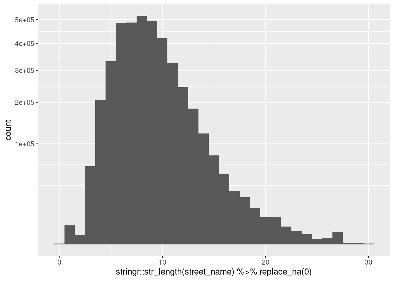
Look at examples of short street names.
# length = 1
d %>%
  dplyr::filter(stringr::str_length(street_name) == 1) %>%
  dplyr::select(starts_with("street_"), res_city_desc) %>%
  dplyr::slice_sample(n = 20) %>%
  gt::gt() %>%
  gt::opt_row_striping() %>%
  gt::tab_style(style = cell_text(weight = "bold"), locations = cells_column_labels()) %>%
gt::fmt_missing(columns = everything(), missing_text = "<NA>")| street_dir | street_name | street_type_cd | street_sufx_cd | res_city_desc |
|---|---|---|---|---|
| <NA> | B | ST | <NA> | FAYETTEVILLE |
| <NA> | E | ST | <NA> | NORTH WILKESBORO |
| W | J | ST | <NA> | ERWIN |
| W | M | ST | <NA> | ERWIN |
| <NA> | C | ST | <NA> | NEW BERN |
| W | B | ST | <NA> | ERWIN |
| <NA> | E | AVE | <NA> | LUMBERTON |
| <NA> | J | ST | <NA> | NORTH WILKESBORO |
| <NA> | J | AVE | <NA> | KURE BEACH |
| W | E | ST | <NA> | ERWIN |
| <NA> | I | ST | <NA> | NORTH WILKESBORO |
| <NA> | A | ST | <NA> | CAMP LEJEUNE |
| <NA> | B | AVE | <NA> | HOT SPRINGS |
| <NA> | A | ST | <NA> | CAMP LEJEUNE |
| S | D | AVE | <NA> | MAIDEN |
| W | F | ST | <NA> | ERWIN |
| <NA> | B | ST | <NA> | FAYETTEVILLE |
| <NA> | K | ST | <NA> | NORTH WILKESBORO |
| W | A | ST | <NA> | KANNAPOLIS |
| <NA> | D | AVE | <NA> | SALISBURY |
# length = 2
d %>%
  dplyr::filter(stringr::str_length(street_name) == 2) %>%
  dplyr::select(starts_with("street_"), res_city_desc) %>%
  dplyr::slice_sample(n = 20) %>%
  gt::gt() %>%
  gt::opt_row_striping() %>%
  gt::tab_style(style = cell_text(weight = "bold"), locations = cells_column_labels()) %>%
gt::fmt_missing(columns = everything(), missing_text = "<NA>")| street_dir | street_name | street_type_cd | street_sufx_cd | res_city_desc |
|---|---|---|---|---|
| <NA> | VI | LN | <NA> | CLAYTON |
| <NA> | RH | RD | <NA> | HICKORY |
| <NA> | DJ | DR | <NA> | STATESVILLE |
| <NA> | 23 | HWY | <NA> | MARS HILL |
| <NA> | LO | DR | <NA> | NEBO |
| E | ST | <NA> | <NA> | ASHEVILLE |
| <NA> | JJ | LN | <NA> | STATESVILLE |
| <NA> | RJ | LN | <NA> | CLINTON |
| <NA> | 63 | HWY | <NA> | HOT SPRINGS |
| <NA> | ST | RD | <NA> | HOLLISTER |
| <NA> | JB | LN | <NA> | BATTLEBORO |
| <NA> | CY | LN | <NA> | RALEIGH |
| <NA> | TJ | TRL | <NA> | HENDERSONVILLE |
| <NA> | KY | FLDS | <NA> | WEAVERVILLE |
| <NA> | 19 | HWY | <NA> | MARS HILL |
| <NA> | CY | LN | <NA> | RALEIGH |
| <NA> | DJ | DR | <NA> | STATESVILLE |
| <NA> | DJ | DR | <NA> | BENSON |
| <NA> | KY | FLDS | <NA> | WEAVERVILLE |
| <NA> | 63 | HWY | <NA> | LEICESTER |
I checked some of these examples against a map.
- Some streets have names like A, B, C, …
- “JC Road” is a valid street name
Look at examples of long street names.
# length >= 28
d %>%
  dplyr::filter(stringr::str_length(street_name) >= 28) %>%
  dplyr::select(starts_with("street_"), res_city_desc) %>%
  dplyr::distinct(.keep_all = TRUE) %>%
  dplyr::arrange(street_name) %>%
  gt::gt() %>%
  gt::opt_row_striping() %>%
  gt::tab_style(style = cell_text(weight = "bold"), locations = cells_column_labels()) %>%
gt::fmt_missing(columns = everything(), missing_text = "<NA>")| street_dir | street_name | street_type_cd | street_sufx_cd | res_city_desc |
|---|---|---|---|---|
| <NA> | BROOKFIELD RETIREMENT CENTER | <NA> | <NA> | LILLINGTON |
| <NA> | CROSS MEMORIAL BAPTIST CHURCH | LOOP | <NA> | MARION |
| <NA> | KINGSDALE MANOR NURSING CENTER | <NA> | <NA> | LUMBERTON |
| <NA> | LOMBARDY VILLAGE MOBILE HOME | PARK | <NA> | LUMBERTON |
| <NA> | LOMBARDY VILLAGE MOBILE HOME | PARK | <NA> | SHANNON |
| <NA> | LOMBARDY VILLAGE MOBILE HOME | PARK | <NA> | REX |
| <NA> | NC HWY 197N NEAR COVY ROCK CHU | <NA> | <NA> | BURNSVILLE |
| <NA> | OLD TAMMANY-OINE ROOKER DAIRY | RD | <NA> | NORLINA |
| <NA> | SWEPSONVILLE-METHODIST CHURCH | RD | <NA> | GRAHAM |
| <NA> | WHEELING VILLAGE TRAILER PARK | <NA> | <NA> | WINSTON SALEM |
| <NA> | WILDLIFE RECREATION AREA ACC | RD | <NA> | LEXINGTON |
| <NA> | WISE-FIVE FORKS- ROBERSON FERR | <NA> | <NA> | MACON |
Long street names are multi-word phrases
- Some appear to have been truncated
4.3 street_type_cd
street_type_cd- Residential address street type (RD, ST, DR, BLVD, etc.)
d %>%
  dplyr::count(street_type_cd) %>%
  dplyr::arrange(desc(n)) %>%
  gt::gt() %>%
  gt::opt_row_striping() %>%
  gt::tab_style(style = cell_text(weight = "bold"), locations = cells_column_labels()) %>%
  gt::fmt_missing(columns = everything(), missing_text = "<NA>") %>%
gt::fmt_number(columns = n, decimals = 0)| street_type_cd | n |
|---|---|
| RD | 1,287,597 |
| DR | 926,884 |
| ST | 512,983 |
| LN | 347,932 |
| CT | 249,682 |
| AVE | 207,808 |
| <NA> | 154,594 |
| CIR | 99,489 |
| PL | 82,253 |
| WAY | 51,625 |
| TRL | 44,565 |
| HWY | 44,189 |
| BLVD | 27,022 |
| LOOP | 9,505 |
| TER | 7,959 |
| PKWY | 6,665 |
| RUN | 5,219 |
| EXT | 4,931 |
| RTE | 2,731 |
| CV | 2,527 |
| PT | 2,263 |
| RDG | 2,124 |
| PARK | 2,013 |
| DORM | 1,756 |
| HTS | 1,684 |
| TRCE | 1,319 |
| BYP | 1,205 |
| SQ | 1,169 |
| PATH | 1,035 |
| VLG | 991 |
| 652 | |
| WALK | 581 |
| CRES | 534 |
| HL | 513 |
| EST | 457 |
| LNDG | 371 |
| ROW | 333 |
| WYND | 328 |
| ALY | 266 |
| HLS | 261 |
| BND | 250 |
| MNR | 222 |
| VW | 217 |
| PLZ | 211 |
| ESTS | 203 |
| HOLW | 200 |
| PASS | 171 |
| BR | 166 |
| XRDS | 163 |
| KNL | 162 |
| CRK | 141 |
| GDNS | 110 |
| MEWS | 102 |
| GRV | 94 |
| MTN | 78 |
| VLY | 67 |
| FLDS | 64 |
| GLN | 61 |
| VIS | 60 |
| SPUR | 58 |
| BRK | 56 |
| KNLS | 51 |
| LK | 51 |
| BLF | 47 |
| COR | 44 |
| HBR | 38 |
| MDWS | 37 |
| SHRS | 33 |
| SPGS | 32 |
| CMN | 28 |
| TRLR | 26 |
| HVN | 24 |
| ANX | 23 |
| CSWY | 22 |
| FRST | 22 |
| PNES | 21 |
| PSGE | 21 |
| CMNS | 20 |
| FLS | 19 |
| IS | 19 |
| CLB | 18 |
| EXPY | 18 |
| LKS | 16 |
| CTR | 15 |
| FRK | 13 |
| TPKE | 13 |
| CRST | 12 |
| SMT | 11 |
| TRAK | 10 |
| FRD | 9 |
| STA | 9 |
| CRSE | 8 |
| FLT | 8 |
| ARC | 7 |
| BRG | 7 |
| ORCH | 7 |
| GDN | 6 |
| GRN | 6 |
| JCT | 6 |
| LDG | 6 |
| SPG | 6 |
| DL | 4 |
| FLTS | 4 |
| FWY | 4 |
| COVE | 3 |
| SHR | 3 |
| FALL | 2 |
| LAND | 2 |
| MDW | 2 |
| MHP | 2 |
| OVAL | 2 |
| RST | 2 |
| VIA | 2 |
| BCH | 1 |
| BTM | 1 |
| DM | 1 |
| FT | 1 |
| RAMP | 1 |
| rd | 1 |
| VL | 1 |
4.4 street_sufx_cd
street_sufx_cd- Residential address street suffix (BUS, EXT, and directional)
d %>%
  dplyr::count(street_sufx_cd) %>%
  dplyr::arrange(desc(n)) %>%
  gt::gt() %>%
  gt::opt_row_striping() %>%
  gt::tab_style(style = cell_text(weight = "bold"), locations = cells_column_labels()) %>%
  gt::fmt_missing(columns = everything(), missing_text = "<NA>") %>%
gt::fmt_number(columns = n, decimals = 0)| street_sufx_cd | n |
|---|---|
| <NA> | 3,941,004 |
| NW | 29,472 |
| SW | 26,587 |
| NE | 24,755 |
| S | 18,870 |
| N | 17,869 |
| W | 13,375 |
| SE | 13,095 |
| E | 13,021 |
| EXT | 1,481 |
| BUS | 169 |
| I | 1 |
5 Locality
res_city_desc- Residential address city name
state_cd- Residential address state code
zip_code- Residential address zip code
d %>%
  dplyr::select(res_city_desc : zip_code) %>%
skimr::skim()| Name | Piped data |
| Number of rows | 4099699 |
| Number of columns | 3 |
| _______________________ | |
| Column type frequency: | |
| character | 3 |
| ________________________ | |
| Group variables | None |
Variable type: character
| skim_variable | n_missing | complete_rate | min | max | empty | n_unique | whitespace |
|---|---|---|---|---|---|---|---|
| res_city_desc | 19 | 1 | 3 | 20 | 0 | 783 | 0 |
| state_cd | 18 | 1 | 2 | 2 | 0 | 5 | 0 |
| zip_code | 21 | 1 | 5 | 9 | 0 | 902 | 0 |
res_city_desc~100% filled (19 missing)state_cd~100% filled (18 missing)zip_code~100% filled (21 missing)
Look at the addresses with any missing locality variable.
d %>%
  dplyr::filter(is.na(res_city_desc) | is.na(state_cd) | is.na(zip_code)) %>%
  dplyr::select(house_num : zip_code) %>%
  dplyr::distinct(.keep_all = TRUE) %>%
  dplyr::arrange(state_cd, res_city_desc, zip_code) %>%
  gt::gt() %>%
  gt::opt_row_striping() %>%
  gt::tab_style(style = cell_text(weight = "bold"), locations = cells_column_labels()) %>%
gt::fmt_missing(columns = everything(), missing_text = "<NA>")| house_num | half_code | street_dir | street_name | street_type_cd | street_sufx_cd | unit_num | res_city_desc | state_cd | zip_code |
|---|---|---|---|---|---|---|---|---|---|
| 5189 | <NA> | <NA> | COVE | RD | <NA> | <NA> | MARION | NC | <NA> |
| 5030 | <NA> | <NA> | COVE | RD | <NA> | <NA> | MARION | NC | <NA> |
| 0 | <NA> | <NA> | H & N MOBILE HOME | PARK | <NA> | <NA> | <NA> | NC | <NA> |
| 0 | <NA> | <NA> | UNKNOWN | <NA> | <NA> | <NA> | <NA> | NC | <NA> |
| 1407 | <NA> | <NA> | OVERLOOK | DR | <NA> | <NA> | LENOIR | <NA> | 28645 |
| 0 | <NA> | <NA> | CONFIDENTIAL | <NA> | <NA> | <NA> | <NA> | <NA> | <NA> |
| 0 | <NA> | <NA> | <NA> | <NA> | <NA> | <NA> | <NA> | <NA> | <NA> |
- Some appear to be good addresses, apart from a missing zip code
- One appears to be a good address, apart from a missing state code
- Some are CONFIDENTIAL addresses, with all details missing
- Some appear to be completely missing the address (homeless persons?)
5.1 res_city_desc
res_city_descResidential address city name
Some city names are very short. Look at the distribution of length of city name.
d %>% pull(res_city_desc) %>% stringr::str_length() %>% summary() Min. 1st Qu. Median Mean 3rd Qu. Max. NA's
3.000 7.000 9.000 8.896 10.000 20.000 19 d %>%
ggplot() +
geom_histogram(aes(x = stringr::str_length(res_city_desc) %>% replace_na(0)), binwidth = 1) +
scale_y_sqrt()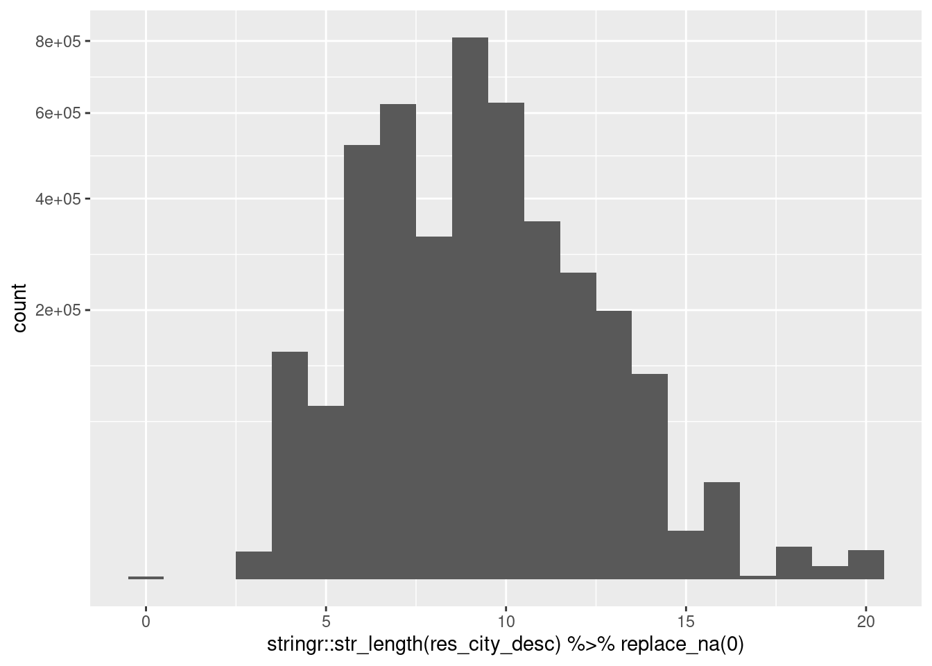
| Version | Author | Date |
|---|---|---|
| ab90fe6 | Ross Gayler | 2021-05-18 |
Look at examples of short city names.
# length = 3
d %>%
  dplyr::filter(stringr::str_length(res_city_desc) == 3) %>%
  dplyr::count(res_city_desc) %>%
  dplyr::slice_sample(n = 20) %>%
  dplyr::arrange(desc(n)) %>%
  gt::gt() %>%
  gt::opt_row_striping() %>%
  gt::tab_style(style = cell_text(weight = "bold"), locations = cells_column_labels()) %>%
  gt::fmt_missing(columns = everything(), missing_text = "<NA>") %>%
gt::fmt_number(columns = n, decimals = 0)| res_city_desc | n |
|---|---|
| ASH | 2,033 |
| REX | 44 |
# length = 4
d %>%
  dplyr::filter(stringr::str_length(res_city_desc) == 4) %>%
  dplyr::count(res_city_desc) %>%
  dplyr::slice_sample(n = 20) %>%
  dplyr::arrange(desc(n)) %>%
  gt::gt() %>%
  gt::opt_row_striping() %>%
  gt::tab_style(style = cell_text(weight = "bold"), locations = cells_column_labels()) %>%
  gt::fmt_missing(columns = everything(), missing_text = "<NA>") %>%
gt::fmt_number(columns = n, decimals = 0)| res_city_desc | n |
|---|---|
| CARY | 56,623 |
| APEX | 20,722 |
| DUNN | 10,964 |
| KING | 7,516 |
| ELON | 5,617 |
| VALE | 4,472 |
| TROY | 4,046 |
| NEBO | 3,311 |
| HAYS | 1,746 |
| STAR | 1,629 |
| OTTO | 1,466 |
| WADE | 1,403 |
| STEM | 1,174 |
| TODD | 940 |
| OLIN | 878 |
| BUNN | 862 |
| GULF | 80 |
| ENKA | 23 |
| LYNN | 8 |
| EARL | 3 |
- These look like plausible place names
Look at examples of long city names.
# length >= 17
d %>%
  dplyr::filter(stringr::str_length(res_city_desc) >= 17) %>%
  dplyr::count(res_city_desc) %>%
  dplyr::slice_sample(n = 20) %>%
  dplyr::arrange(desc(n)) %>%
  gt::gt() %>%
  gt::opt_row_striping() %>%
  gt::tab_style(style = cell_text(weight = "bold"), locations = cells_column_labels()) %>%
  gt::fmt_missing(columns = everything(), missing_text = "<NA>") %>%
gt::fmt_number(columns = n, decimals = 0)| res_city_desc | n |
|---|---|
| BOILING SPRING LAKES | 2,370 |
| WRIGHTSVILLE BEACH | 1,434 |
| RUTHERFORD COLLEGE | 724 |
| LEWISTON WOODVILLE | 668 |
| NORTH TOPSAIL BEACH | 451 |
| LITTLE SWITZERLAND | 155 |
| CONNELLYS SPRINGS | 35 |
- Long city names are multi-word phrases
5.2 state_cd
state_cd- Residential address state code
d %>%
  dplyr::count(state_cd) %>%
  dplyr::arrange(desc(n)) %>%
  gt::gt() %>%
  gt::opt_row_striping() %>%
  gt::tab_style(style = cell_text(weight = "bold"), locations = cells_column_labels()) %>%
  gt::fmt_missing(columns = everything(), missing_text = "<NA>") %>%
gt::fmt_number(columns = n, decimals = 0)| state_cd | n |
|---|---|
| NC | 4,099,631 |
| TN | 29 |
| <NA> | 18 |
| GA | 13 |
| VA | 7 |
| SC | 1 |
Residential state codes are almost entirely NC (North Carolina)
- There are a small number in neighbouring states (non-resident voters?)
5.3 zip_code
zip_code Residential address zip code
The zip codes are not all the same length. Look at the distribution of length of zip code
d %>%
  dplyr::select(zip_code) %>%
  dplyr::mutate(length = stringr::str_length(zip_code)) %>%
  dplyr::count(length) %>%
  gt::gt() %>%
  gt::opt_row_striping() %>%
  gt::tab_style(style = cell_text(weight = "bold"), locations = cells_column_labels()) %>%
  gt::fmt_missing(columns = everything(), missing_text = "<NA>") %>%
gt::fmt_number(columns = n, decimals = 0)| length | n |
|---|---|
| 5 | 4,099,667 |
| 9 | 11 |
| <NA> | 21 |
Look at the 9-digit zip codes.
d %>%
  dplyr::filter(stringr::str_length(zip_code) == 9) %>%
  dplyr::select(street_name : zip_code) %>%
  dplyr::arrange(zip_code) %>%
  gt::gt() %>%
  gt::opt_row_striping() %>%
  gt::tab_style(style = cell_text(weight = "bold"), locations = cells_column_labels()) %>%
gt::fmt_missing(columns = everything(), missing_text = "<NA>")| street_name | street_type_cd | street_sufx_cd | unit_num | res_city_desc | state_cd | zip_code |
|---|---|---|---|---|---|---|
| ECHO | LN | <NA> | <NA> | SANFORD | NC | 273308492 |
| UNKNOWN | <NA> | <NA> | <NA> | LILLINGTON | NC | 275468949 |
| LINCOLN MCKAY | DR | <NA> | <NA> | LILLINGTON | NC | 275469001 |
| SMITH | ST | <NA> | <NA> | ALBEMARLE | NC | 280014351 |
| INDIAN MOUND | RD | <NA> | <NA> | ALBEMARLE | NC | 280019245 |
| POND | ST | <NA> | <NA> | ALBEMARLE | NC | 280019766 |
| NC 731 HWY | <NA> | <NA> | B | NORWOOD | NC | 281289420 |
| FRIENDLY MCLEOD | LN | <NA> | <NA> | DUNN | NC | 283349250 |
| BEAVER DAM | RD | <NA> | <NA> | ERWIN | NC | 283399790 |
| WIRE | RD | <NA> | <NA> | LINDEN | NC | 283569413 |
| WALKER | RD | <NA> | <NA> | LINDEN | NC | 283569416 |
- The addresses with 9-digit zipcodes look plausible
- 5-digit and 9-digit zip codes are
valid
6 Telephone
area_cd- Area code for phone numberphone_num- Telephone number
d %>%
  dplyr::select(area_cd, phone_num) %>%
skimr::skim()| Name | Piped data |
| Number of rows | 4099699 |
| Number of columns | 2 |
| _______________________ | |
| Column type frequency: | |
| character | 2 |
| ________________________ | |
| Group variables | None |
Variable type: character
| skim_variable | n_missing | complete_rate | min | max | empty | n_unique | whitespace |
|---|---|---|---|---|---|---|---|
| area_cd | 2628117 | 0.36 | 1 | 3 | 0 | 507 | 0 |
| phone_num | 2540990 | 0.38 | 1 | 7 | 0 | 1072592 | 0 |
- Area code ~36% filled
- Phone number ~38% filled
Look at the relationship between missing area code and missing phone number.
table(area_miss = is.na(d$area_cd), phone_miss = is.na(d$phone_num)) phone_miss
area_miss FALSE TRUE
FALSE 1449568 22014
TRUE 109141 2518976- Area code and phone number are generally missing together, but …
- Area code is frequently missing even when phone number is present (possibly assumed to be a local number)
- Phone number is less frequently missing when area code is present (possibly assumed to be in the local area, but phone number unknown)
6.1 area_cd
area_cd- Area code for phone number
Look at some area code examples grouped by length, where there is a phone number.
d %>%
  dplyr::filter(!is.na(phone_num)) %>%
  dplyr::count(area_cd) %>% # count occurrences of each unique value
  dplyr::mutate(length = stringr::str_length(area_cd) %>% replace_na(0)) %>%
  dplyr::group_by(length) %>%
  dplyr::slice_max(order_by = n, n = 10, with_ties = FALSE) %>%
  gt::gt() %>%
  gt::opt_row_striping() %>%
  gt::tab_style(style = cell_text(weight = "bold"), locations = cells_column_labels()) %>%
  gt::fmt_missing(columns = everything(), missing_text = "<NA>") %>%
gt::fmt_number(columns = n, decimals = 0)| area_cd | n |
|---|---|
| 0 | |
| <NA> | 109,141 |
| 2 | |
| 70 | 1 |
| 91 | 1 |
| 3 | |
| 828 | 356,621 |
| 910 | 345,033 |
| 252 | 216,848 |
| 704 | 208,035 |
| 919 | 170,862 |
| 336 | 131,018 |
| 999 | 4,824 |
| 980 | 1,386 |
| 000 | 1,291 |
| 757 | 967 |
- Many records with phone numbers are missing area code.
- Area codes less than 3 characters long are probably typos.
- Area code “999” and “000” are probably missing.
6.2 phone_num
phone_num- Telephone number
Look at some phone number examples grouped by length, where there is a phone number.
d %>%
  dplyr::filter(!is.na(phone_num)) %>%
  dplyr::count(phone_num) %>% # count occurrences of each unique value
  dplyr::mutate(length = stringr::str_length(phone_num) %>% replace_na(0)) %>%
  dplyr::group_by(length) %>%
  dplyr::slice_max(order_by = n, n = 5, with_ties = FALSE) %>%
  gt::gt() %>%
  gt::opt_row_striping() %>%
  gt::tab_style(style = cell_text(weight = "bold"), locations = cells_column_labels()) %>%
  gt::fmt_missing(columns = everything(), missing_text = "<NA>") %>%
gt::fmt_number(columns = n, decimals = 0)| phone_num | n |
|---|---|
| 1 | |
| - | 14 |
| 0 | 1 |
| 6 | 1 |
| 9 | 1 |
| 3 | |
| 299 | 1 |
| 368 | 1 |
| 372 | 1 |
| 562 | 1 |
| 565 | 1 |
| 4 | |
| -221 | 1 |
| -644 | 1 |
| -691 | 1 |
| -700 | 1 |
| -708 | 1 |
| 5 | |
| 11959 | 1 |
| 26108 | 1 |
| 61974 | 1 |
| 89054 | 1 |
| 6 | |
| 089909 | 1 |
| 324171 | 1 |
| 335788 | 1 |
| 335940 | 1 |
| 349803 | 1 |
| 7 | |
| 0000000 | 9,671 |
| 9999999 | 6,282 |
| 5244446 | 182 |
| 4975411 | 108 |
| 2987911 | 94 |
- Phone numbers less than 7 characters long are probably typos.
- Phone numbers “0000000” and “9999999” are probably missing.
Timing
Computation time (excl. render): 398.496 sec elapsed
sessionInfo()R version 4.1.0 (2021-05-18)
Platform: x86_64-pc-linux-gnu (64-bit)
Running under: Ubuntu 20.10
Matrix products: default
BLAS: /usr/lib/x86_64-linux-gnu/blas/libblas.so.3.9.0
LAPACK: /usr/lib/x86_64-linux-gnu/lapack/liblapack.so.3.9.0
locale:
[1] LC_CTYPE=en_AU.UTF-8 LC_NUMERIC=C
[3] LC_TIME=en_AU.UTF-8 LC_COLLATE=en_AU.UTF-8
[5] LC_MONETARY=en_AU.UTF-8 LC_MESSAGES=en_AU.UTF-8
[7] LC_PAPER=en_AU.UTF-8 LC_NAME=C
[9] LC_ADDRESS=C LC_TELEPHONE=C
[11] LC_MEASUREMENT=en_AU.UTF-8 LC_IDENTIFICATION=C
attached base packages:
[1] stats graphics grDevices datasets utils methods base
other attached packages:
[1] tidyr_1.1.3 skimr_2.1.3 ggplot2_3.3.3 forcats_0.5.1
[5] lubridate_1.7.10 vroom_1.4.0 stringr_1.4.0 gt_0.3.0
[9] dplyr_1.0.6 fs_1.5.0 here_1.0.1 tictoc_1.0.1
[13] targets_0.4.2
loaded via a namespace (and not attached):
[1] Rcpp_1.0.6 ps_1.6.0 rprojroot_2.0.2 digest_0.6.27
[5] utf8_1.2.1 R6_2.5.0 repr_1.1.3 backports_1.2.1
[9] evaluate_0.14 highr_0.9 pillar_1.6.1 rlang_0.4.11
[13] data.table_1.14.0 whisker_0.4 callr_3.7.0 jquerylib_0.1.4
[17] checkmate_2.0.0 rmarkdown_2.8 labeling_0.4.2 igraph_1.2.6
[21] bit_4.0.4 munsell_0.5.0 compiler_4.1.0 httpuv_1.6.1
[25] xfun_0.23 pkgconfig_2.0.3 base64enc_0.1-3 htmltools_0.5.1.1
[29] tidyselect_1.1.1 tibble_3.1.2 bookdown_0.22 workflowr_1.6.2
[33] codetools_0.2-18 fansi_0.4.2 crayon_1.4.1 withr_2.4.2
[37] later_1.2.0 grid_4.1.0 jsonlite_1.7.2 gtable_0.3.0
[41] lifecycle_1.0.0 git2r_0.28.0 magrittr_2.0.1 scales_1.1.1
[45] cli_2.5.0 stringi_1.6.2 farver_2.1.0 renv_0.13.2
[49] promises_1.2.0.1 bslib_0.2.5 ellipsis_0.3.2 generics_0.1.0
[53] vctrs_0.3.8 tools_4.1.0 bit64_4.0.5 glue_1.4.2
[57] purrr_0.3.4 processx_3.5.2 parallel_4.1.0 yaml_2.2.1
[61] colorspace_2.0-1 knitr_1.33 sass_0.4.0