06_class_pair_synthetic_score.Rmd
Ross Gayler
2023-02-06
Last updated: 2023-02-25
Checks: 7 0
Knit directory: multiclass_AUC/
This reproducible R Markdown analysis was created with workflowr (version 1.7.0). The Checks tab describes the reproducibility checks that were applied when the results were created. The Past versions tab lists the development history.
Great! Since the R Markdown file has been committed to the Git repository, you know the exact version of the code that produced these results.
Great job! The global environment was empty. Objects defined in the global environment can affect the analysis in your R Markdown file in unknown ways. For reproduciblity it’s best to always run the code in an empty environment.
The command set.seed(20230112) was run prior to running
the code in the R Markdown file. Setting a seed ensures that any results
that rely on randomness, e.g. subsampling or permutations, are
reproducible.
Great job! Recording the operating system, R version, and package versions is critical for reproducibility.
Nice! There were no cached chunks for this analysis, so you can be confident that you successfully produced the results during this run.
Great job! Using relative paths to the files within your workflowr project makes it easier to run your code on other machines.
Great! You are using Git for version control. Tracking code development and connecting the code version to the results is critical for reproducibility.
The results in this page were generated with repository version 17ee60b. See the Past versions tab to see a history of the changes made to the R Markdown and HTML files.
Note that you need to be careful to ensure that all relevant files for
the analysis have been committed to Git prior to generating the results
(you can use wflow_publish or
wflow_git_commit). workflowr only checks the R Markdown
file, but you know if there are other scripts or data files that it
depends on. Below is the status of the Git repository when the results
were generated:
Ignored files:
    Ignored:    .Rhistory
    Ignored:    .Rproj.user/
    Ignored:    renv/library/
    Ignored:    renv/sandbox/
    Ignored:    renv/staging/
Note that any generated files, e.g. HTML, png, CSS, etc., are not included in this status report because it is ok for generated content to have uncommitted changes.
These are the previous versions of the repository in which changes were
made to the R Markdown
(analysis/06_class_pair_synthetic_score.Rmd) and HTML
(docs/06_class_pair_synthetic_score.html) files. If you’ve
configured a remote Git repository (see ?wflow_git_remote),
click on the hyperlinks in the table below to view the files as they
were in that past version.
| File | Version | Author | Date | Message |
|---|---|---|---|---|
| Rmd | 17ee60b | Ross Gayler | 2023-02-25 | Publish notebook 06 |
| Rmd | 0451805 | Ross Gayler | 2023-02-24 | end 2023-02-24 |
Dependencies
Read the saved example data.
d_scores <- readRDS(file = here::here("output", "d_scores.RDS")) |>
  # convert case, class_id and score_id to integer factors for safety & better label order
  dplyr::mutate(
    case = forcats::as_factor(case),
    class_id = forcats::as_factor(class_id),
    score_id = forcats::as_factor(score_id)
  )
Introduction
Classic SDT has two classes discriminated by a single score. Multiclass classification typically has as many scores per observation as there are classes, with the observation being predicted as belonging to the class with the highest score. This leads to difficulty in mapping the multiclass scenario into the SDT conceptual framework.
For each case characterised by the vector of observations \(x\) there should be a score (\(s_i(x)\)) for each class \(i\). Normatively, each class score (\(s_i(x)\)) should be some fixed monotonic function of the probability (\(p( class = i \mid x)\)) of the observation belonging to class \(i\). In principle, we can transform the score \(s_i(x)\) to the estimated probability \(\hat{p}_i(class = i \mid x)\) and use that estimated probability as the score. Note that I am explicitly stating that \(\hat{p}_i(x)\) is derived from \(s_i(x)\). The literature tends to be somewhat sketchy about this and unclear as to whether the probabilities are derived from scores of the data or are somehow Platonic ideal probabilities that exist independent of the scores.
The Hand and Till (2001) multiclass AUC approach works by breaking the multiclass problem into all pairs of classes to be discriminated, calculating a discriminability measure (AUC) for each pair of classes, then averaging that pairwise discriminability across the set of class pairs. For each pair of classes, \(i\) and \(j\), they calculate the AUC for discriminating the classes separately by \(s_i(x)\) and \(s_j(x)\), then average those two AUC values to get the AUC for the class pair. I believe that this approach, while useful, is not correct because the use of the scores in the AUC calculation does not correspond to the way they are used in the classifier. In classic SDT a single score is compared to a fixed threshold. This corresponds to the way the scores are used in the Hand and Till calculation. However, the classifiers we are interested in take two scores per case (one for each of the two classes in the pair) and assign the case to the class with the higher score. That is, the classification algorithm compares two scores to each other rather than one score to a fixed threshold.
Another perspective on this point is that the AUC calculation conceptually involves independently selecting one case at random from each of the two classes and calculating the score for each case. The scores are independent in that they are based on separate cases. In contrast, the classifier as implemented takes one case (from some class) and calculates both scores from the same case. The scores are not independent because they are calculated from the same case.
It can be demonstrated that considering the two scores in isolation does not guarantee a good assessment of the performance of the classifier. Assume that each of the class scores is reasonably discriminating of class membership. This ensures that the AUC calculated by the Hand and Till method is reasonably high. However, it is possible for the two class scores to be calibrated differently to the outcome. (We observed this empirically in an earlier notebook.) In the extreme case there could be no overlap between the ranges of the two scores, so that the score for one class was always greater than the score for the other class, regardless of the true class for the case. This would mean that the classifier, as implemented, was useless for discriminating the classes, even though each class score was reasonably discriminating.
We need some way of assessing the performance of the classifier as implemented (i.e. depending on the comparison of the two class scores). We attempt to do this by creating a synthetic score that captures the relationship between the two class scores and allows us to apply the classic SDT conceptual model of, for each case, comparing the single synthetic score to a fixed threshold. The constraints are:
- For each case, combine the two class scores into a single synthetic score, and
- For each case, comparison of the synthetic score to a fixed threshold must yield the same assigned class that would have been obtained by comparing the two class scores.
There is also another constraint (ability to simulate response bias) that we will deal with in detail in a later notebook.
The objective of this notebook is to make some empirical attempts at creating a synthetic score to illustrate the issues that arise. This is not intended as an exhaustive analysis of the datasets, so the datasets and classes to analyse will be chosen for convenience.
Dataset: UCR_14, Model: MINIROCKET, Classes: 1 & 3
Analysis is more technically difficult with smaller numbers of cases, so choose UCR_14 rather than UCR_48. Analysis is more technically difficult with greater discriminability, so choose MINIROCKET rather than HDC_MINIROCKET.
Choose classes 1 and 3 because an earlier notebook showed that these classes had lower separability compared to other pairs of classes. Also, it looked like class score 1 and class score 3 behaved differently, which is interesting.
Restrict the data to only those cases belonging to class 1 or class
3. Then reformat the data so that there is one row per case with both
class scores present in the same row. Also, create the score difference
(score_diff) as an obvious candidate for a synthetic
score.
d <- d_scores |>
  dplyr::filter(dataset == "UCR_14" & model == "MINIROCKET") |>
  dplyr::filter(class_id %in% c(1, 3) & score_id %in% c(1, 3)) |>
  tidyr::pivot_wider(
    id_cols = c(dataset, model, case, class_id),
    names_from = score_id,
    values_from = score_val,
    names_prefix = "score_"
  ) |>
  dplyr::mutate(score_diff = score_1 - score_3)
summary(d)
dataset model case class_id
Length:685 Length:685 1 : 1 1 :343
Class :character Class :character 2 : 1 3 :342
Mode :character Mode :character 4 : 1 0 : 0
5 : 1 2 : 0
7 : 1 4 : 0
8 : 1 5 : 0
(Other):679 (Other): 0
score_1 score_3 score_diff
Min. :-1.36849 Min. :-1.5579 Min. :-2.3371
1st Qu.:-0.54931 1st Qu.:-0.9123 1st Qu.:-0.9598
Median :-0.06212 Median :-0.5472 Median : 0.4780
Mean :-0.06124 Mean :-0.2890 Mean : 0.2277
3rd Qu.: 0.48664 3rd Qu.: 0.4646 3rd Qu.: 1.3211
Max. : 1.44485 Max. : 1.1561 Max. : 2.9160
First look at each of the two class scores (score_1 and
score_3) as predictors in isolation. This parallels their
use in Hand and Till (2001). Then look at
some potential synthetic scores.
score_1
Look at score_1 as a predictor of class_id.
This includes calculating the AUC of the score as a predictor of the
class, using the equivalence to the Mann-Whitney-Wilcoxon test statistic
noted in Hand and Till (2001).
Look at the distribution of score_1 by
class_id.
n_pairs <- d$class_id |> as.integer() |> table() |> prod() # get the number of pairs of class_i,class_j cases

auc <- wilcox.test(d$score_1[d$class_id == 1], d$score_1[d$class_id == 3])$statistic / n_pairs

ggplot(d) +
  geom_density(aes(x = score_1, fill = class_id), alpha = 0.5) +
  labs(
    title = "UCR_14 MINIROCKET, Classes 1 & 3",
    subtitle = glue::glue("Score 1, AUC = {round(auc, 3)}")
  )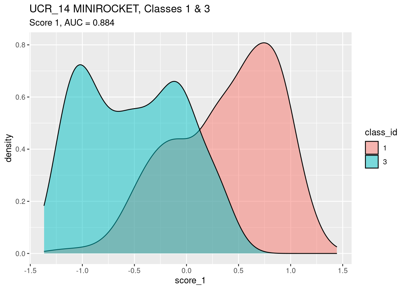
- Score 1 is a reasonable discriminator of class
- There is a lump of class 1 cases that have an intermediate (~ 0)
value of
score_1. - There is a considerable lump of class 3 cases that have an
intermediate (~ 0) value of
score_1.
Look at the calibration of score_1 as a predictor of
class_id.
Fit a smooth calibration curve.
fit <- mgcv::gam(class_id == 1 ~ s(score_1) + 1, family = binomial(), data = d)
summary(fit)
Family: binomial
Link function: logit

Formula:
class_id == 1 ~ s(score_1) + 1

Parametric coefficients:
            Estimate Std. Error z value Pr(>|z|)
(Intercept)   0.7061     0.3374   2.093   0.0363 *
---
Signif. codes:  0 '***' 0.001 '**' 0.01 '*' 0.05 '.' 0.1 ' ' 1

Approximate significance of smooth terms:
            edf Ref.df Chi.sq p-value
s(score_1) 4.92  5.889  112.1  <2e-16 ***
---
Signif. codes:  0 '***' 0.001 '**' 0.01 '*' 0.05 '.' 0.1 ' ' 1

R-sq.(adj) =  0.466   Deviance explained = 43.3%
UBRE = -0.19686  Scale est. = 1         n = 685
plot(fit)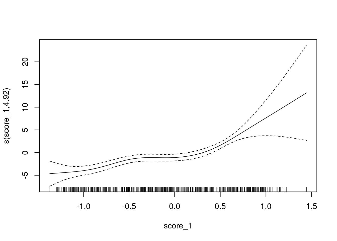
The y axis is scaled as log-odds of being class 1 versus class 3.
- The calibration curve is monotonic.
- There is a flat segment covering the score range of approximately \([-0.5, 0.1]\). In this score range the probability of the case being from class 1 is constant despite the increasing score.
Fit a linear calibration as being close enough for current purposes.
fit <- mgcv::gam(class_id == 1 ~ score_1 + 1, family = binomial(), data = d)
summary(fit)
Family: binomial
Link function: logit

Formula:
class_id == 1 ~ score_1 + 1

Parametric coefficients:
            Estimate Std. Error z value Pr(>|z|)
(Intercept)   0.1805     0.1045   1.726   0.0843 .
score_1       3.2015     0.2349  13.631   <2e-16 ***
---
Signif. codes:  0 '***' 0.001 '**' 0.01 '*' 0.05 '.' 0.1 ' ' 1


R-sq.(adj) =  0.438   Deviance explained = 39.2%
UBRE = -0.15115 Scale est. = 1 n = 685- The slope is 3.2, that is, the log-odds of being from class 1 increases by 3.2 per unit increase in score 1.
score_3
Look at score_3 as a predictor of
class_id.
auc <- wilcox.test(d$score_3[d$class_id == 3], d$score_3[d$class_id == 1])$statistic / n_pairs

ggplot(d) +
  geom_density(aes(x = score_3, fill = class_id), alpha = 0.5) +
  labs(
    title = "UCR_14 MINIROCKET, Classes 1 & 3",
    subtitle = glue::glue("Score 3, AUC = {round(auc, 3)}")
  )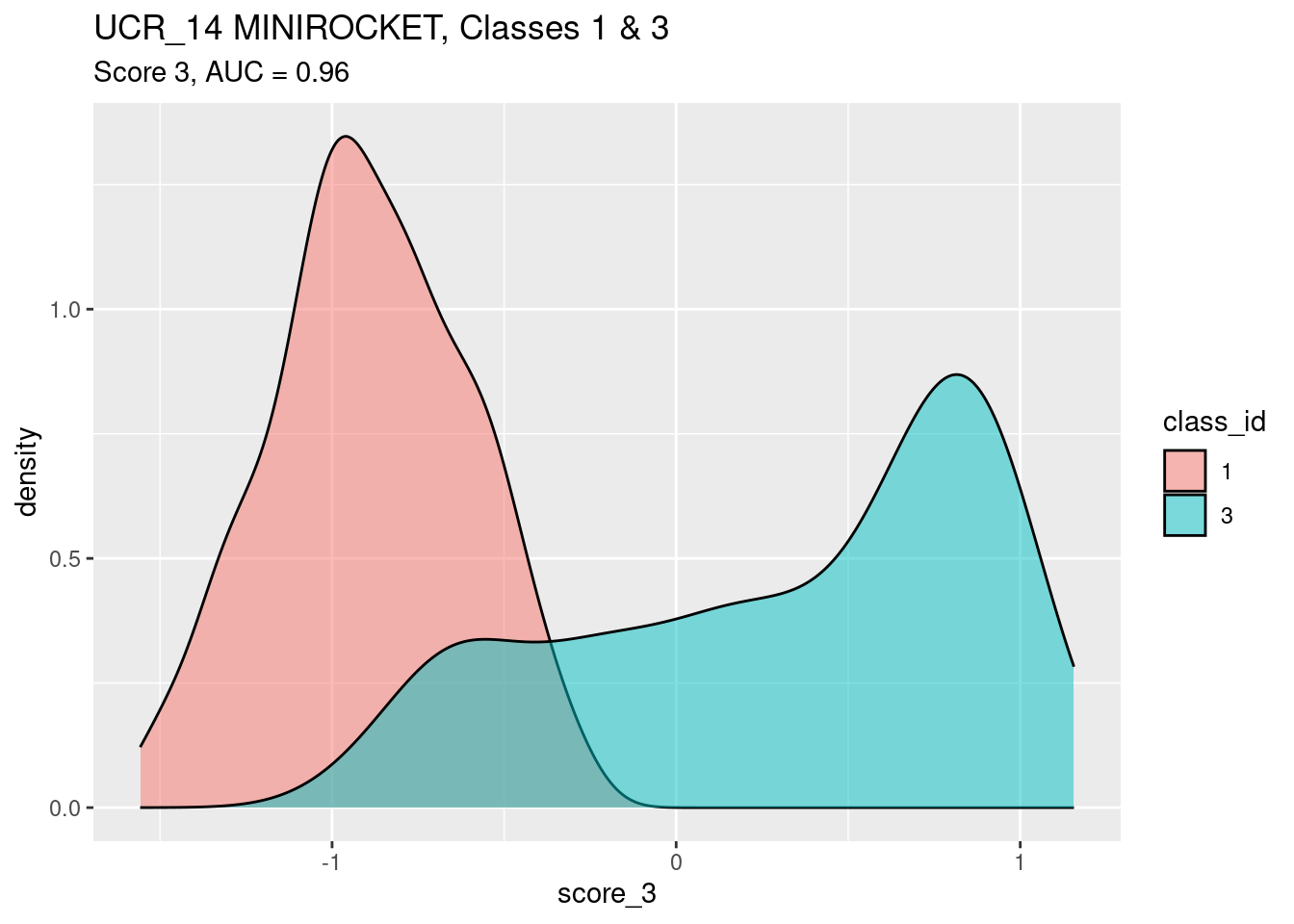
- Score 3 is a good discriminator of class
- Score 3 is a better discriminator of classes 1 and 3 than score 1.
- There is a lump of class 3 cases that have an intermediate (~ -0.5)
value of
score_3. - Score 3 is probably a better discriminator than score 1 because there is no lump of off-target cases getting intermediate values of the score.
Look at the calibration of score_3 as a predictor of
class_id.
Fit a smooth calibration curve.
fit <- mgcv::gam(class_id == 1 ~ s(score_3) + 1, family = binomial(), data = d)
summary(fit)
Family: binomial
Link function: logit

Formula:
class_id == 1 ~ s(score_3) + 1

Parametric coefficients:
            Estimate Std. Error z value Pr(>|z|)
(Intercept)   -5.523      4.881  -1.132    0.258

Approximate significance of smooth terms:
             edf Ref.df Chi.sq p-value
s(score_3) 3.639   4.26  59.84  <2e-16 ***
---
Signif. codes:  0 '***' 0.001 '**' 0.01 '*' 0.05 '.' 0.1 ' ' 1

R-sq.(adj) =  0.711   Deviance explained = 68.1%
UBRE = -0.54362  Scale est. = 1         n = 685
plot(fit)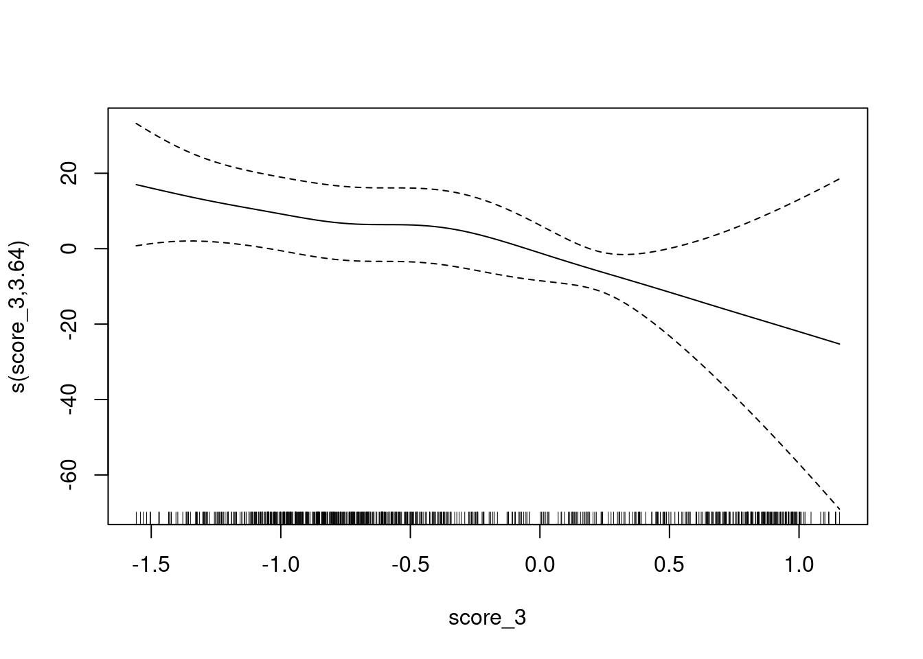
The y axis is still scaled as log-odds of being class 1 versus class 3 (rather than class 3 versus class 1). It is convenient to do this because later we will be using both scores to predict one outcome, so the outcome may as well be the same for all models.
- The calibration curve has negative slope because we are using score 3 to predict class 1. This does not cause any problems because the two outcome classes are complementary.
- The calibration curve is monotonic.
- There is a flat segment covering the score range of approximately \([-0.8, 0.5]\). In this score range the probability of the case being from class 1 is constant despite the increasing score.
Fit a linear calibration as being close enough for current purposes.
fit <- mgcv::gam(class_id == 1 ~ score_3 + 1, family = binomial(), data = d)
summary(fit)
Family: binomial
Link function: logit

Formula:
class_id == 1 ~ score_3 + 1

Parametric coefficients:
            Estimate Std. Error z value Pr(>|z|)
(Intercept)  -2.8959     0.3499  -8.277   <2e-16 ***
score_3      -6.1673     0.5583 -11.047   <2e-16 ***
---
Signif. codes:  0 '***' 0.001 '**' 0.01 '*' 0.05 '.' 0.1 ' ' 1


R-sq.(adj) =  0.695   Deviance explained = 65.9%
UBRE = -0.52156 Scale est. = 1 n = 685- The slope is -6.2, that is, the log-odds of being from class 1 decreases by 6.2 per unit increase in score 3.
- The magnitude of the slope is quite a different from score 1.
- This implies that the calibrations of the scores are quite different,
- which further implies that the performance of the classifier as implemented is not as good as it could be, because score 1 and score 3 are not measured on the same scale.
score_diff
The difference between the two scores looks like a reasonable attempt at a synthetic score. The sign of the difference indicates which score (out of score 1 and score 3) is greater. Comparing the score difference to a fixed threshold of zero leads to the same assigned class obtained by assigning the class corresponding to the larger score in the classifier as implemented.
Look at score_diff as a predictor of
class_id.
auc <- wilcox.test(d$score_diff[d$class_id == 1], d$score_diff[d$class_id == 3])$statistic / n_pairs

ggplot(d) +
  geom_vline(xintercept = 0) +
  geom_density(aes(x = score_diff, fill = class_id), alpha = 0.5) +
  labs(
    title = "UCR_14 MINIROCKET, Classes 1 & 3",
    subtitle = glue::glue("Score score_diff, AUC = {round(auc, 3)}")
  )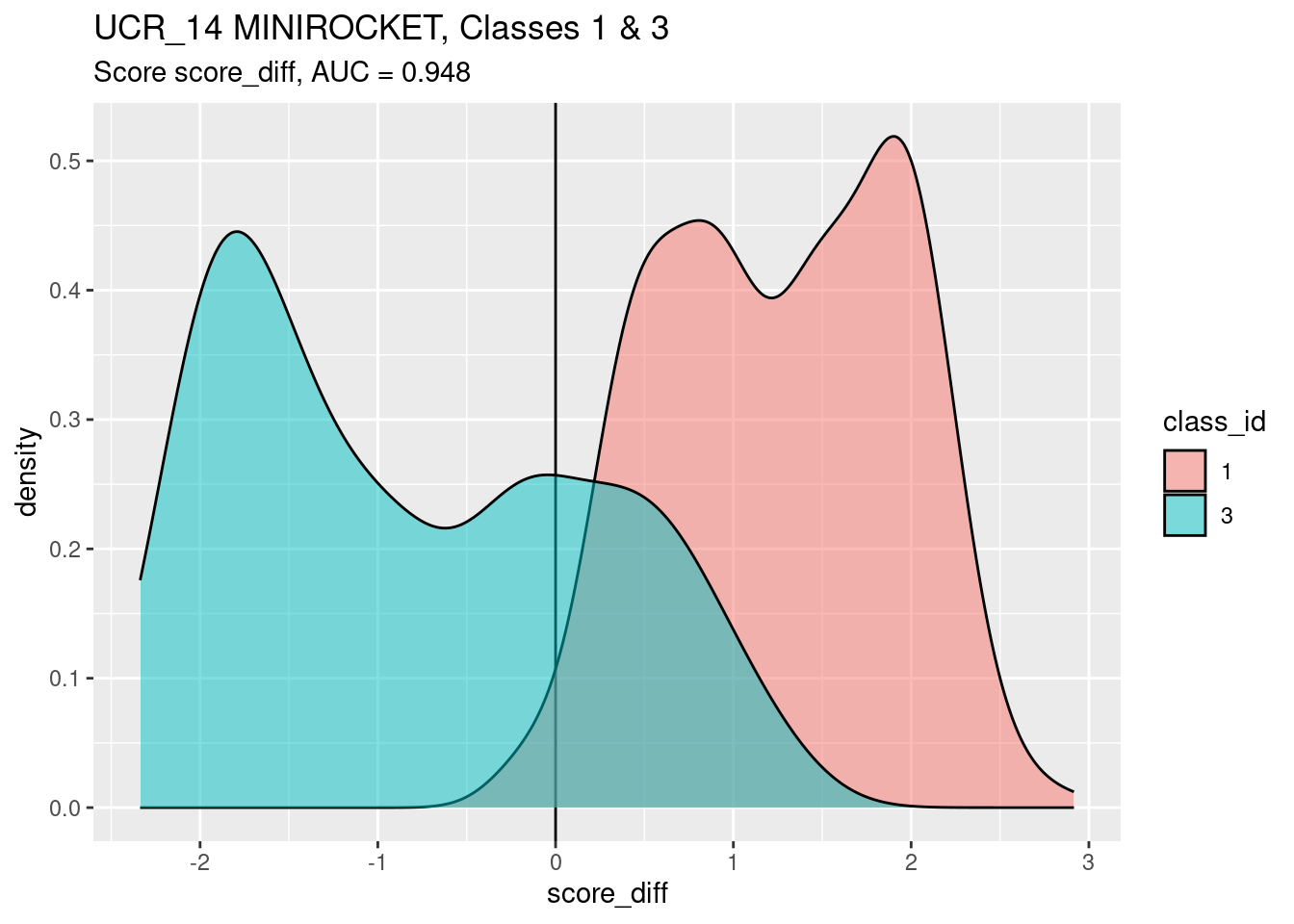
The calculated AUC accurately reflects the ability of
score_diff to discriminate classes 1 and 3. However, I am
not convinced that score_diff is the best synthetic score
to summarise the behaviour of the classifier as implemented, because I
suspect that the score difference does not accurately capture the
behaviour of the classifier under varying response bias.
score_diffis a good discriminator of classscore_diffis a better discriminator of classes 1 and 3 than score 1.score_diffis a slightly worse discriminator of classes 1 and 3 than score 3.- I suspect that this slight decrement in performance is due (at least, in part) to the differing calibration between the two class scores.
- There are lumps of class 1 and class 3 cases having intermediate score values.
- There is a sizeable fraction of the class 3 cases falling above the zero threshold. These cases are misclassified as belonging to class 1.
Look at the calibration of score_diff as a predictor of
class_id.
Fit a smooth calibration curve.
fit <- mgcv::gam(class_id == 1 ~ s(score_diff) + 1, family = binomial(), data = d)
summary(fit)
Family: binomial
Link function: logit

Formula:
class_id == 1 ~ s(score_diff) + 1

Parametric coefficients:
            Estimate Std. Error z value Pr(>|z|)
(Intercept)   -1.765      1.727  -1.022    0.307

Approximate significance of smooth terms:
                edf Ref.df Chi.sq p-value
s(score_diff) 3.681  4.435  76.23  <2e-16 ***
---
Signif. codes:  0 '***' 0.001 '**' 0.01 '*' 0.05 '.' 0.1 ' ' 1

R-sq.(adj) =  0.647   Deviance explained = 62.2%
UBRE = -0.46178  Scale est. = 1         n = 685
plot(fit)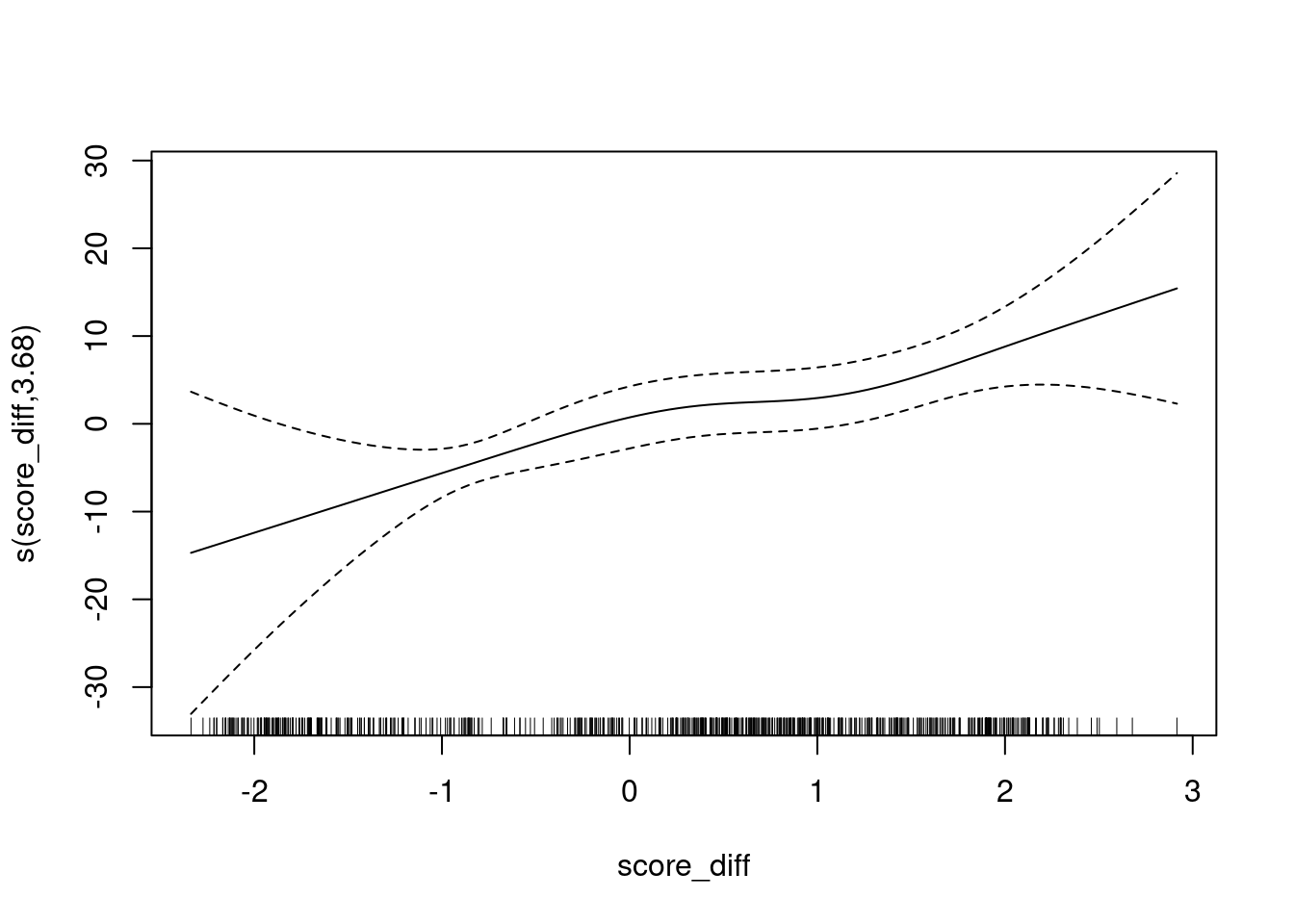
The y axis is scaled as log-odds of being class 1 versus class 3.
- The calibration curve has positive slope because the sign of the score indicates score 1 is greater than score 3 and we are predicting score 1.
- The calibration curve is monotonic.
- The slope is less in the score range of approximately \([0.3, 1]\).
Fit a linear calibration as being close enough for current purposes.
fit <- mgcv::gam(class_id == 1 ~ score_diff + 1, family = binomial(), data = d)
summary(fit)
Family: binomial
Link function: logit

Formula:
class_id == 1 ~ score_diff + 1

Parametric coefficients:
            Estimate Std. Error z value Pr(>|z|)
(Intercept)  -1.2032     0.1842  -6.533 6.43e-11 ***
score_diff    2.9417     0.2535  11.606  < 2e-16 ***
---
Signif. codes:  0 '***' 0.001 '**' 0.01 '*' 0.05 '.' 0.1 ' ' 1


R-sq.(adj) =  0.637   Deviance explained = 60.5%
UBRE = -0.44604 Scale est. = 1 n = 685- The slope is 2.9.
- There is no point comparing this slope to the slopes of the other scores as it is not compared to the other scores in the classifier as implemented.
score_1 + score_3
In this subsection I will construct a new synthetic score that is an optimal linear composite of score 1 and score 3. I will use logistic regression to find the weighting of the two scores that best predicts the true class. Note that this synthetic score is not guaranteed to emulate the classifier as implemented at the current response bias. The only weighted sum for which that is true is the score difference (weights of +1 and -1, and isomorphic transforms). The reason for constructing this score is to investigate whether it is possible to combine the class scores in a way which is more predictive than the individual scores and the classifier as implemented.
Fit a model to predict the true class from a linear composite of score 1 and score 3.
fit <- mgcv::gam(class_id == 1 ~ score_1 + score_3 + 1, family = binomial(), data = d)
summary(fit)
Family: binomial
Link function: logit

Formula:
class_id == 1 ~ score_1 + score_3 + 1

Parametric coefficients:
            Estimate Std. Error z value Pr(>|z|)
(Intercept)  -2.7370     0.3554  -7.700 1.36e-14 ***
score_1       0.8903     0.3901   2.282   0.0225 *
score_3      -5.7334     0.5805  -9.877  < 2e-16 ***
---
Signif. codes:  0 '***' 0.001 '**' 0.01 '*' 0.05 '.' 0.1 ' ' 1


R-sq.(adj) =  0.698   Deviance explained = 66.5%
UBRE = -0.52627 Scale est. = 1 n = 685- The deviance explained (66.5%) is slightly higher than for the linear fit to score 3 alone (65.9%) indicating that the combined model is slightly more predictive (as measured by goodness of fit).
Add the synthetic score to the data frame.
d$score_sum <- predict(fit)
summary(d)
dataset model case class_id
Length:685 Length:685 1 : 1 1 :343
Class :character Class :character 2 : 1 3 :342
Mode :character Mode :character 4 : 1 0 : 0
5 : 1 2 : 0
7 : 1 4 : 0
8 : 1 5 : 0
(Other):679 (Other): 0
score_1 score_3 score_diff score_sum
Min. :-1.36849 Min. :-1.5579 Min. :-2.3371 Min. :-10.4169
1st Qu.:-0.54931 1st Qu.:-0.9123 1st Qu.:-0.9598 1st Qu.: -5.8154
Median :-0.06212 Median :-0.5472 Median : 0.4780 Median : 0.4405
Mean :-0.06124 Mean :-0.2890 Mean : 0.2277 Mean : -1.1346
3rd Qu.: 0.48664 3rd Qu.: 0.4646 3rd Qu.: 1.3211 3rd Qu.: 2.8014
Max. : 1.44485 Max. : 1.1561 Max. : 2.9160 Max. : 7.0613
Look at score_sum as a predictor of
class_id.
auc <- wilcox.test(d$score_sum[d$class_id == 1], d$score_sum[d$class_id == 3])$statistic / n_pairs

ggplot(d) +
  geom_vline(xintercept = 0) +
  geom_density(aes(x = score_sum, fill = class_id), alpha = 0.5) +
  labs(
    title = "UCR_14 MINIROCKET, Classes 1 & 3",
    subtitle = glue::glue("Score score_sum, AUC = {round(auc, 3)}")
  )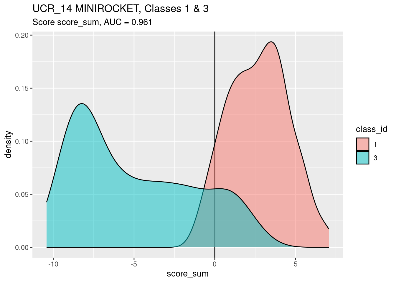
score_sumis a slightly better discriminator (by AUC) of classes 1 and 3 than score 3.
Look at the calibration of score_sum as a predictor of
class_id.
Fit a smooth calibration curve.
fit <- mgcv::gam(class_id == 1 ~ s(score_sum) + 1, family = binomial(), data = d)
summary(fit)
Family: binomial
Link function: logit

Formula:
class_id == 1 ~ s(score_sum) + 1

Parametric coefficients:
            Estimate Std. Error z value Pr(>|z|)
(Intercept)   -6.854      6.600  -1.038    0.299

Approximate significance of smooth terms:
               edf Ref.df Chi.sq p-value
s(score_sum) 3.739    4.3  51.56  <2e-16 ***
---
Signif. codes:  0 '***' 0.001 '**' 0.01 '*' 0.05 '.' 0.1 ' ' 1

R-sq.(adj) =  0.714   Deviance explained = 68.8%
UBRE = -0.55334  Scale est. = 1         n = 685
plot(fit)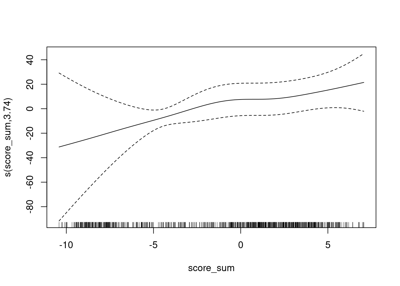
The y axis is scaled as log-odds of being class 1 versus class 3.
- The calibration curve is monotonic.
- The slope is less in the score range of approximately \([0, 2]\).
Fit a linear calibration as being close enough for current purposes.
fit <- mgcv::gam(class_id == 1 ~ score_sum + 1, family = binomial(), data = d)
summary(fit)
Family: binomial
Link function: logit

Formula:
class_id == 1 ~ score_sum + 1

Parametric coefficients:
              Estimate Std. Error z value Pr(>|z|)
(Intercept) -8.842e-15  1.525e-01     0.0        1
score_sum    1.000e+00  9.171e-02    10.9   <2e-16 ***
---
Signif. codes:  0 '***' 0.001 '**' 0.01 '*' 0.05 '.' 0.1 ' ' 1


R-sq.(adj) =  0.698   Deviance explained = 66.5%
UBRE = -0.52918 Scale est. = 1 n = 685- The slope is 1 and intercept 0, because this model had been fit with a logistic regression and we are not performing this current regression on a different data set.
s(score_1, score_3)
In this subsection I will construct a new synthetic score that is a smooth function of the joint values of score 1 and score 3. This will be even more predictive of the true class than the linear composite of the scores if there is an interaction present. The reason for constructing this score is to investigate whether it is possible to combine the class scores in a way which is more predictive than the classifier as implemented.
Fit a model to predict the true class from a smooth joint function of score 1 and score 3.
fit <- mgcv::gam(class_id == 1 ~ s(score_1, score_3) + 1, family = binomial(), data = d)
summary(fit)
Family: binomial
Link function: logit

Formula:
class_id == 1 ~ s(score_1, score_3) + 1

Parametric coefficients:
            Estimate Std. Error z value Pr(>|z|)
(Intercept)   -3.516      5.183  -0.678    0.498

Approximate significance of smooth terms:
                     edf Ref.df Chi.sq  p-value
s(score_1,score_3) 14.09  16.51   54.3 8.16e-06 ***
---
Signif. codes:  0 '***' 0.001 '**' 0.01 '*' 0.05 '.' 0.1 ' ' 1

R-sq.(adj) =  0.748   Deviance explained = 73.3%
UBRE = -0.58612  Scale est. = 1         n = 685
plot(fit)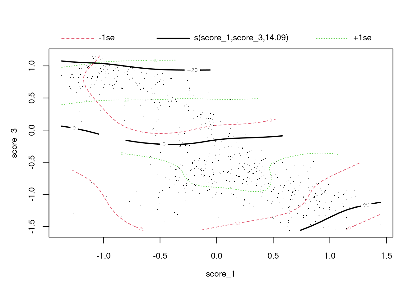
- The deviance explained (73.3%) is higher than for the previous scores, indicating that the combined model is more predictive (as measured by goodness of fit).
The plot shows the surface of log-odds of being class 1 versus class 3. The solid black lines are contours of the surface. The dashed red and green lines are confidence intervals around the contours. The dots are the cases.
- For high values of score 3 (> -0.5) the contours are
approximately parallel to the score 1 axis, indicating that the log-odds
of true class depends almost entirely on score 3 and does not vary with
score 1.
- Increasing score 3 indicates decreasing log-odds of being class 1.
- For low values of score 3 (< -0.5) the contour line slopes up to
the right, indicating that the log-odds of true class depends on both
score 3 and score 1.
- Increasing score 3 indicates decreasing log-odds of being class 1.
- Increasing score 1 indicates increasing log-odds of being class 1.
Add the synthetic score to the data frame.
d$score_intx <- predict(fit)
summary(d)
dataset model case class_id
Length:685 Length:685 1 : 1 1 :343
Class :character Class :character 2 : 1 3 :342
Mode :character Mode :character 4 : 1 0 : 0
5 : 1 2 : 0
7 : 1 4 : 0
8 : 1 5 : 0
(Other):679 (Other): 0
score_1 score_3 score_diff score_sum
Min. :-1.36849 Min. :-1.5579 Min. :-2.3371 Min. :-10.4169
1st Qu.:-0.54931 1st Qu.:-0.9123 1st Qu.:-0.9598 1st Qu.: -5.8154
Median :-0.06212 Median :-0.5472 Median : 0.4780 Median : 0.4405
Mean :-0.06124 Mean :-0.2890 Mean : 0.2277 Mean : -1.1346
3rd Qu.: 0.48664 3rd Qu.: 0.4646 3rd Qu.: 1.3211 3rd Qu.: 2.8014
Max. : 1.44485 Max. : 1.1561 Max. : 2.9160 Max. : 7.0613
score_intx
Min. :-24.9999
1st Qu.:-15.4271
Median : 0.3357
Mean : -3.5157
3rd Qu.: 3.7874
Max. : 21.2899
Look at score_intx as a predictor of
class_id.
auc <- wilcox.test(d$score_intx[d$class_id == 1], d$score_intx[d$class_id == 3])$statistic / n_pairs

ggplot(d) +
  geom_vline(xintercept = 0) +
  geom_density(aes(x = score_intx, fill = class_id), alpha = 0.5) +
  labs(
    title = "UCR_14 MINIROCKET, Classes 1 & 3",
    subtitle = glue::glue("Score score_intx, AUC = {round(auc, 3)}")
  )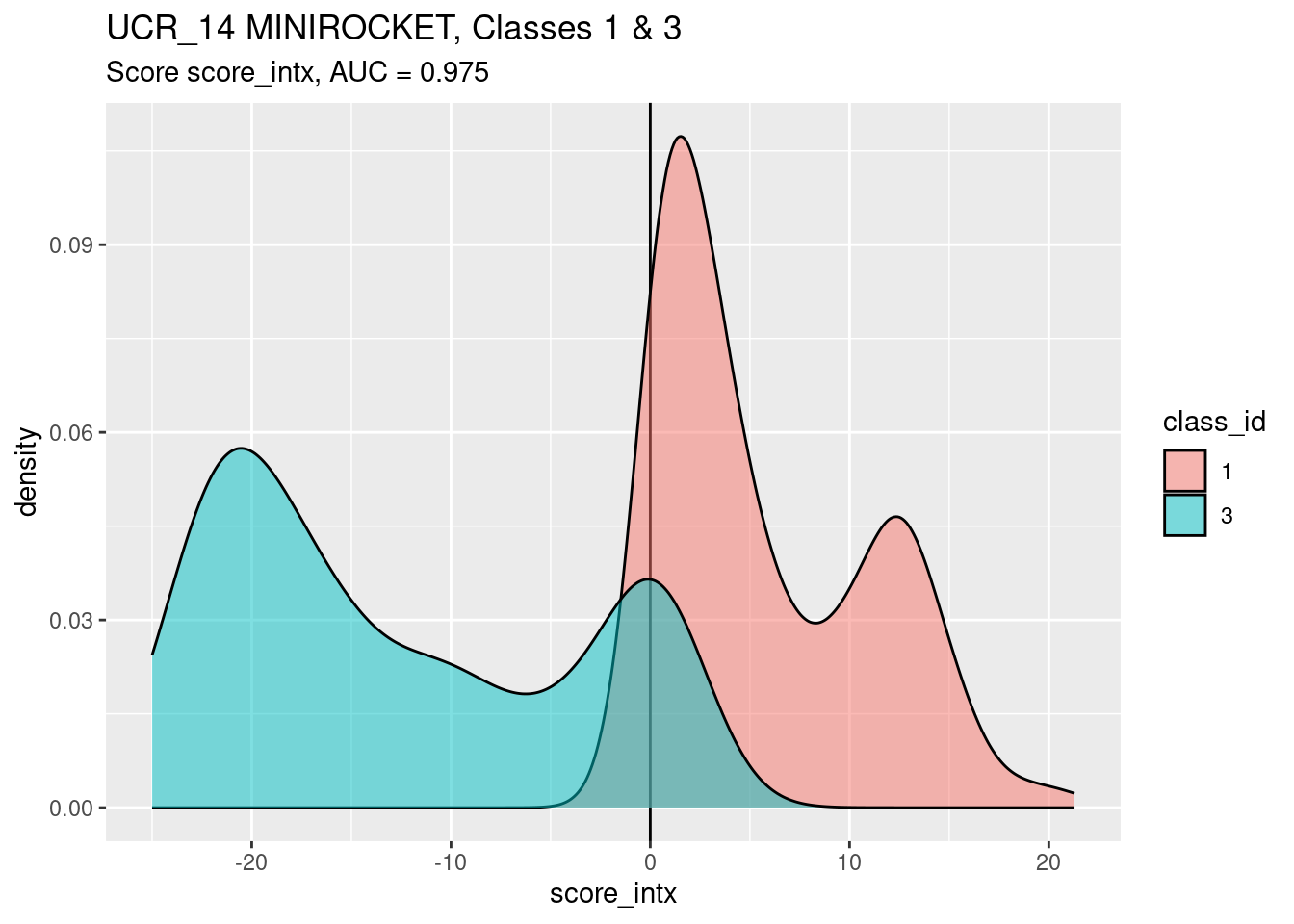
score_intxis a better discriminator (by AUC) of classes 1 and 3 than the other scores examined.- There are significant lumps of class 1 and class 3 cases in the ambiguous region around the threshold score value of zero.
Look at the calibration of score_intx as a predictor of
class_id.
Fit a smooth calibration curve.
fit <- mgcv::gam(class_id == 1 ~ s(score_intx) + 1, family = binomial(), data = d)
summary(fit)
Family: binomial
Link function: logit

Formula:
class_id == 1 ~ s(score_intx) + 1

Parametric coefficients:
            Estimate Std. Error z value Pr(>|z|)
(Intercept)  -3.9604     0.6701   -5.91 3.42e-09 ***
---
Signif. codes:  0 '***' 0.001 '**' 0.01 '*' 0.05 '.' 0.1 ' ' 1

Approximate significance of smooth terms:
              edf Ref.df Chi.sq p-value
s(score_intx)   1      1  48.55  <2e-16 ***
---
Signif. codes:  0 '***' 0.001 '**' 0.01 '*' 0.05 '.' 0.1 ' ' 1

R-sq.(adj) =  0.752   Deviance explained = 73.4%
UBRE = -0.62509  Scale est. = 1         n = 685
plot(fit)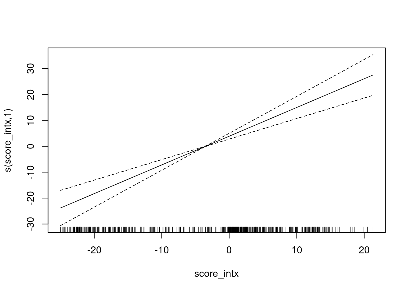
Fit a linear calibration as being close enough for current purposes.
fit <- mgcv::gam(class_id == 1 ~ score_intx + 1, family = binomial(), data = d)
summary(fit)
Family: binomial
Link function: logit

Formula:
class_id == 1 ~ score_intx + 1

Parametric coefficients:
            Estimate Std. Error z value Pr(>|z|)
(Intercept) -0.06493    0.18045  -0.360    0.719
score_intx   1.10801    0.15787   7.018 2.24e-12 ***
---
Signif. codes:  0 '***' 0.001 '**' 0.01 '*' 0.05 '.' 0.1 ' ' 1


R-sq.(adj) =  0.752   Deviance explained = 73.4%
UBRE = -0.62509 Scale est. = 1 n = 685- The slope is 1.1 (rather than 1) and intercept 0.
- I suspect the calibration is not quite exact because there are some approximations in the fitting of the spline surface.
Summary
- Calculating the AUC with respect to the class scores in isolation is not compatible with the way the scores are used in the classifier as implemented.
- The class scores in a class pair can differ considerably in how well they discriminate the classes.
- The class scores are not necessarily well calibrated to the log-odds of true class.
- The calibration can differ considerably between class scores.
- Comparison of class scores in the classifier as implemented can be less discriminating than the individual class scores.
- The average of the class score discriminability is not necessarily a good summary of the performance of the classifier as implemented.
- Class scores can be combined to give a synthetic score which can be compared to a fixed threshold, as in classic SDT.
- Some synthetic scores can be more discriminating than the class scores in isolation.
- Some synthetic scores can emulate the class assignments to cases of the classifier as implemented.
References
sessionInfo()R version 4.2.2 Patched (2022-11-10 r83330)
Platform: x86_64-pc-linux-gnu (64-bit)
Running under: Ubuntu 22.04.2 LTS
Matrix products: default
BLAS: /usr/lib/x86_64-linux-gnu/blas/libblas.so.3.10.0
LAPACK: /usr/lib/x86_64-linux-gnu/lapack/liblapack.so.3.10.0
locale:
[1] LC_CTYPE=en_AU.UTF-8 LC_NUMERIC=C
[3] LC_TIME=en_AU.UTF-8 LC_COLLATE=en_AU.UTF-8
[5] LC_MONETARY=en_AU.UTF-8 LC_MESSAGES=en_AU.UTF-8
[7] LC_PAPER=en_AU.UTF-8 LC_NAME=C
[9] LC_ADDRESS=C LC_TELEPHONE=C
[11] LC_MEASUREMENT=en_AU.UTF-8 LC_IDENTIFICATION=C
attached base packages:
[1] stats graphics grDevices datasets utils methods base
other attached packages:
[1] mgcv_1.8-41 nlme_3.1-161 glue_1.6.2 ggplot2_3.4.0
[5] tidyr_1.3.0 forcats_0.5.2 dplyr_1.0.10 here_1.0.1
[9] workflowr_1.7.0
loaded via a namespace (and not attached):
[1] tidyselect_1.2.0 xfun_0.36 bslib_0.4.2 purrr_1.0.1
[5] splines_4.2.2 lattice_0.20-45 colorspace_2.1-0 vctrs_0.5.2
[9] generics_0.1.3 htmltools_0.5.4 yaml_2.3.7 utf8_1.2.2
[13] rlang_1.0.6 jquerylib_0.1.4 later_1.3.0 pillar_1.8.1
[17] withr_2.5.0 lifecycle_1.0.3 stringr_1.5.0 munsell_0.5.0
[21] gtable_0.3.1 evaluate_0.20 labeling_0.4.2 knitr_1.42
[25] callr_3.7.3 fastmap_1.1.0 httpuv_1.6.8 ps_1.7.2
[29] fansi_1.0.4 highr_0.10 Rcpp_1.0.10 renv_0.16.0
[33] promises_1.2.0.1 scales_1.2.1 cachem_1.0.6 jsonlite_1.8.4
[37] farver_2.1.1 fs_1.6.0 digest_0.6.31 stringi_1.7.12
[41] processx_3.8.0 getPass_0.2-2 rprojroot_2.0.3 grid_4.2.2
[45] cli_3.6.0 tools_4.2.2 magrittr_2.0.3 sass_0.4.5
[49] tibble_3.1.8 whisker_0.4.1 pkgconfig_2.0.3 ellipsis_0.3.2
[53] Matrix_1.5-3 rmarkdown_2.20 httr_1.4.4 rstudioapi_0.14
[57] R6_2.5.1 git2r_0.30.1 compiler_4.2.2