Characterise Simulation Data (Single Target)

workflowr

• Summary
• Checks
• Past versions

Last updated: 2021-08-18

Checks: 7 0

Knit directory: VSA_altitude_hold/

This reproducible R Markdown analysis was created with workflowr (version 1.6.2). The Checks tab describes the reproducibility checks that were applied when the results were created. The Past versions tab lists the development history.

---

R Markdown file: up-to-date

Great! Since the R Markdown file has been committed to the Git repository, you know the exact version of the code that produced these results.

Environment: empty

Great job! The global environment was empty. Objects defined in the global environment can affect the analysis in your R Markdown file in unknown ways. For reproduciblity it’s best to always run the code in an empty environment.

Seed: set.seed(20210617)

The command set.seed(20210617) was run prior to running the code in the R Markdown file. Setting a seed ensures that any results that rely on randomness, e.g. subsampling or permutations, are reproducible.

Session information: recorded

Great job! Recording the operating system, R version, and package versions is critical for reproducibility.

Cache: none

Nice! There were no cached chunks for this analysis, so you can be confident that you successfully produced the results during this run.

File paths: relative

Great job! Using relative paths to the files within your workflowr project makes it easier to run your code on other machines.

Repository version: af002d9

Great! You are using Git for version control. Tracking code development and connecting the code version to the results is critical for reproducibility.

The results in this page were generated with repository version af002d9. See the Past versions tab to see a history of the changes made to the R Markdown and HTML files.

Note that you need to be careful to ensure that all relevant files for the analysis have been committed to Git prior to generating the results (you can use wflow_publish or wflow_git_commit). workflowr only checks the R Markdown file, but you know if there are other scripts or data files that it depends on. Below is the status of the Git repository when the results were generated:

Ignored files:
    Ignored:    .Rhistory
    Ignored:    .Rproj.user/
    Ignored:    renv/library/
    Ignored:    renv/local/
    Ignored:    renv/staging/

Note that any generated files, e.g. HTML, png, CSS, etc., are not included in this status report because it is ok for generated content to have uncommitted changes.

---

These are the previous versions of the repository in which changes were made to the R Markdown (analysis/characterise_single_target_data.Rmd) and HTML (docs/characterise_single_target_data.html) files. If you’ve configured a remote Git repository (see ?wflow_git_remote), click on the hyperlinks in the table below to view the files as they were in that past version.

File	Version	Author	Date	Message
Rmd	867778a	Ross Gayler	2021-08-11	Add multi target simulation data
html	867778a	Ross Gayler	2021-08-11	Add multi target simulation data

---

This notebook characterises data generated by the simulation of the classically implemented altitude hold controller. We need to understand the properties of the signals in order to design VSA implementations of them. This set of simulation data files has a single target altitude that is constant within each simulation. The duration of each simulation is 5 seconds.

The values to be characterised are all the real scalars corresponding to the nodes in the data flow diagram for Design 01.

1 Data

• The data is generated from runs of the classically implemented simulation.

• The data files are stored in the data/single_target directory.

• The data is supplied as CSV files, each file corresponding to a different run of the simulation.

• Each run of the simulation corresponds to a set of starting conditions, parameters, and program details.

• The name of each data file contains the values of all the starting conditions, parameters, and program details.

• The only starting condition that varies between runs is the initial altitude. The multicopter is released at the starting height and the multicopter must command the motors to attain the target altitude.

• In this set of data files the target altitude parameter is always 5 metres and constant over the duration of the simulation. More generally this should be treated as a demand which can vary with time.

• The other parameters are tuning constants (\(k_p\), \(k_i\), and \(k_{windup}\)) for the PID controller and are constant across runs of the simulation.

• The program details that vary between simulation runs correspond to our evolving understanding of the details of the system and the requirements of this analysis.

  • The \(uclip\) program detail indicates whether the motor demand value (\(u\)) has been clipped to the the range \([0, 1]\) prior to export. The clipped value is what is used to drive command the motors. However, the unclipped value is more useful for comparing to the mathematically reconstructed value of the other nodes.

    • The \(uclip\) program detail can be interpreted as indicating whether the clipped or unclipped value has been exported. \(uclip = TRUE\) corresponds to exporting the value of the \(u\) node of the data flow diagram for Design 01. \(uclip = FALSE\) corresponds to exporting the value of the node \(i7\).

  • The \(dz0\) program detail indicates whether the vertical velocity (\(dz\)) is zero on the first recorded time step.

    • The simulation is based on OpenAI Gym which has a “convention of having the reset() function call the step() function, which updates the state and returns the new state, reward, and a flag for whether the game is over”. This was used to intialise the simulations (\(dz0 = FALSE\)), with the result that the state update was run as part of the initialisation. This isn’t particularly significant except that the starting state of the simulation is not quite what you might expect. This was fixed in later simulation runs (\(dz0 = TRUE\)).

• Each row of the data file corresponds to a point in time and successive rows correspond to successive points in time. (This is a discrete time simulation with fixed time steps of 10ms.)

• Each file contains 500 time steps of 10ms (i.e. 5s total).

• Each column of the data file corresponds to a node of the data flow diagram.

• Only a subset of the nodes are supplied (\(z\), \(dz\), \(e\), \(ei\), and \(u\) - the nodes in rectangular boxes in the DFD supplied by Simon Levy) and the values of the other nodes can be reconstructed mathematically.

• The values supplied from the input files are recorded to three decimal places, so there is scope for approximation error due to the limited precision.

• Where a node value is supplied from the input file and that node also has upstream nodes in the DFD the supplied and calculated values should be equal and can be compared.

  • For nodes like this, in this notebook I will use the imported value rather than the calculatedt value as the input for downstream nodes in order to avoid propagating approximation errors.

1.1 Read data

Read the data from the simulations and mathematically reconstruct the values of the nodes not included in the input files.

# function to clip value to a range
clip <- function(
  x, # numeric
  x_min, # numeric[1] - minimum output value
  x_max  # numeric[1] - maximum output value
) # value # numeric - x constrained to the range [x_min, x_max]
  {
  x %>% pmax(x_min) %>% pmin(x_max)
}

# function to extract a numeric parameter value from the file name
get_param_num <- function(
  file, # character - vector of file names
  regexp # character[1] - regular expression for "param=value"
         # use a capture group to get the value part
) # value # numeric - vector of parameter values
{
  file %>% str_match(regexp) %>% 
      subset(select = 2) %>% as.numeric()
}

# function to extract a logical parameter value from the file name
get_param_log <- function(
  file, # character - vector of file names
  regexp # character[1] - regular expression for "param=value"
  # use a capture group to get the value part
  # value *must* be T or F
) # value # logical - vector of logical parameter values
{
  file %>% str_match(regexp) %>% 
    subset(select = 2) %>% as.character() %>% "=="("T")
}

# read the data
d_wide <- fs::dir_ls(path = here::here("data", "single_target"), regexp = "/k_start=.*\\.csv$") %>% # get file paths
  vroom::vroom(id = "file") %>% # read files
  dplyr::mutate( # add extra columns
    file = file %>% fs::path_ext_remove() %>% fs::path_file(), # get file name
    # get parameters
    k_start  = file %>% get_param_num("k_start=([.0-9]+)"), 
    k_p      = file %>% get_param_num("kp=([.0-9]+)"),
    k_i      = file %>% get_param_num("Ki=([.0-9]+)"),
    k_tgt    = file %>% get_param_num("k_tgt=([.0-9]+)"),
    k_windup = file %>% get_param_num("k_windup=([.0-9]+)"),
    uclip    = file %>% get_param_log("_uclip=([TF])"),
    dz0      = file %>% get_param_log("_dz0=([TF])"),
    # Deal with the fact that the interpretation of the imported u value
    # depends on the uclip parameter
    u_import = u, # keep a copy of the imported value to one side
    u = dplyr::if_else(uclip, # make u the "correct" value
                       u_import, 
                       clip(u_import, 0, 1)
                       ),
    # reconstruct the missing nodes
    i1 = k_tgt - z,
    i2 = i1 - dz,
    i3 = e * k_p,
    i9 = lag(ei, n = 1, default = 0), # initialised to zero
    i4 = e + i9,
    i5 = i4 %>% clip(-k_windup, k_windup),
    i6 = ei * k_i,
    i7 = i3 + i6,
    i8 = i7 %>% clip(0, 1)
  ) %>% 
  # add time variable per file
  dplyr::group_by(file) %>% 
  dplyr::mutate(t = 1:n()) %>% 
  dplyr::ungroup()

Rows: 3500 Columns: 6

── Column specification ────────────────────────────────────────────────────────
Delimiter: ","
dbl (5): z, dz, e, ei, u

ℹ Use `spec()` to retrieve the full column specification for this data.
ℹ Specify the column types or set `show_col_types = FALSE` to quiet this message.

dplyr::glimpse(d_wide)

Rows: 3,500
Columns: 24
$ file     <chr> "k_start=10.00_k_tgt=5.00_kp=0.20_Ki=3.00_k_windup=0.20_uclip…
$ z        <dbl> 10.000, 9.999, 9.998, 9.995, 9.992, 9.987, 9.982, 9.975, 9.96…
$ dz       <dbl> -0.058, -0.156, -0.254, -0.352, -0.450, -0.548, -0.646, -0.74…
$ e        <dbl> -4.942, -4.843, -4.744, -4.643, -4.542, -4.439, -4.335, -4.23…
$ ei       <dbl> -0.2, -0.2, -0.2, -0.2, -0.2, -0.2, -0.2, -0.2, -0.2, -0.2, -…
$ u        <dbl> 0, 0, 0, 0, 0, 0, 0, 0, 0, 0, 0, 0, 0, 0, 0, 0, 0, 0, 0, 0, 0…
$ k_start  <dbl> 10, 10, 10, 10, 10, 10, 10, 10, 10, 10, 10, 10, 10, 10, 10, 1…
$ k_p      <dbl> 0.2, 0.2, 0.2, 0.2, 0.2, 0.2, 0.2, 0.2, 0.2, 0.2, 0.2, 0.2, 0…
$ k_i      <dbl> 3, 3, 3, 3, 3, 3, 3, 3, 3, 3, 3, 3, 3, 3, 3, 3, 3, 3, 3, 3, 3…
$ k_tgt    <dbl> 5, 5, 5, 5, 5, 5, 5, 5, 5, 5, 5, 5, 5, 5, 5, 5, 5, 5, 5, 5, 5…
$ k_windup <dbl> 0.2, 0.2, 0.2, 0.2, 0.2, 0.2, 0.2, 0.2, 0.2, 0.2, 0.2, 0.2, 0…
$ uclip    <lgl> TRUE, TRUE, TRUE, TRUE, TRUE, TRUE, TRUE, TRUE, TRUE, TRUE, T…
$ dz0      <lgl> FALSE, FALSE, FALSE, FALSE, FALSE, FALSE, FALSE, FALSE, FALSE…
$ u_import <dbl> 0, 0, 0, 0, 0, 0, 0, 0, 0, 0, 0, 0, 0, 0, 0, 0, 0, 0, 0, 0, 0…
$ i1       <dbl> -5.000, -4.999, -4.998, -4.995, -4.992, -4.987, -4.982, -4.97…
$ i2       <dbl> -4.942, -4.843, -4.744, -4.643, -4.542, -4.439, -4.336, -4.23…
$ i3       <dbl> -0.9884, -0.9686, -0.9488, -0.9286, -0.9084, -0.8878, -0.8670…
$ i9       <dbl> 0.0, -0.2, -0.2, -0.2, -0.2, -0.2, -0.2, -0.2, -0.2, -0.2, -0…
$ i4       <dbl> -4.942, -5.043, -4.944, -4.843, -4.742, -4.639, -4.535, -4.43…
$ i5       <dbl> -0.2, -0.2, -0.2, -0.2, -0.2, -0.2, -0.2, -0.2, -0.2, -0.2, -…
$ i6       <dbl> -0.6, -0.6, -0.6, -0.6, -0.6, -0.6, -0.6, -0.6, -0.6, -0.6, -…
$ i7       <dbl> -1.5884, -1.5686, -1.5488, -1.5286, -1.5084, -1.4878, -1.4670…
$ i8       <dbl> 0, 0, 0, 0, 0, 0, 0, 0, 0, 0, 0, 0, 0, 0, 0, 0, 0, 0, 0, 0, 0…
$ t        <int> 1, 2, 3, 4, 5, 6, 7, 8, 9, 10, 11, 12, 13, 14, 15, 16, 17, 18…

1.2 Check data

Check the data for consistency.

1.2.1 Initial values

The different starting conditions correspond to the multicopter being dropped/released at different altitudes.

Time \(t = 1\) should correspond to the moment of release. At that time the altitude should be exactly the starting altitude and the vertical velocity (\(dz\)) should be exactly zero (but we know it wasn’t in the \(dz0 = FALSE\) simulations).

Treating propagation through the DFD as instantaneous, we can calculate the values of the internal nodes as a function of the imposed initial values of the imported nodes. The internal nodes are generally functions of the values at the same time. However, the nodes involved in the calculation of the integrated errors (\(ei\)) are functions of the integrated error at the previous time step. This means that there is a dependency on the initial value of \(ei\) (which is initialised to zero in the simulation code)

Check the initial node values imported from the simulations.

d_wide %>% 
  dplyr::filter(t == 1) %>% # get initial time step
  dplyr::arrange(k_start, dz0, uclip) %>% 
  dplyr::select(file, k_tgt, k_start, z, dz0, dz, e, ei, u) %>% 
  DT::datatable(rownames = FALSE)

• As expected, the initial altitude (\(z\)) is equal to (\(k_{start}\)) for all simulations.

• As expected, The initial vertical velocities (\(dz\)) are zero when \(dz0 = TRUE\) and nonzero otherwise. As explained earlier this is due to the use of reset() to initialise the simulations.

• As expected, the error \(e\) and integrated error \(ei\) are nonzero at the first time step because the starting altitudes are not equal to the target altitude and because of the instantaneous propagation of values through the DFD. The correctness of the values will be checked in the next section.

• As expected, the motor command \(u\) is nonzero when the starting altitude is below the target (because the multicopter has to climb to the target) and zero when the starting altitude is above the target (because the multicopter has to fall to the target). The correctness of the values will be checked in the next section.

1.2.2 Check calculated values

Where possible, compare the calculated values with the values imported from the simulator. The calculated nodes which can be checked against the imported reference values are: e, ei, u.

The analyses below involve calculating the distributions of values over the available time steps. This is a slightly odd interpretation of distribution in that the available time steps do not constitute a sample from some stationary distribution. Rather, the values should be interpreted as roughly representative of the multicopter’s response to a perturbation.

1.2.2.1 e = i2

\(e\) and \(i2\) should be identical (up to approximation error).

d_wide %>% 
  dplyr::group_by(file) %>% 
  dplyr::summarise(
    min = min(e - i2) %>% round(3),
    p01 = quantile(e - i2, probs = 0.01) %>% round(3), #1st percentile
    p50 = median(e - i2) %>% round(3),
    p99 = quantile(e - i2, probs = 0.99) %>% round(3), # 99th percentile
    max = max(e - i2) %>% round(3)
  ) %>% 
  DT::datatable(rownames = FALSE, caption = "*** e - i2 ***")

• The imported and reconstructed values agree except for approximation error due to the low precision of the numbers in the files.

1.2.2.2 ei = i5

\(ei\) and \(i5\) should be identical (up to approximation error).

d_wide %>% 
  dplyr::group_by(file) %>% 
  dplyr::summarise(
    min = min(ei - i5) %>% round(3),
    p01 = quantile(ei - i5, probs = 0.01) %>% round(3), #1st percentile
    p50 = median(ei - i5) %>% round(3),
    p99 = quantile(ei - i5, probs = 0.99) %>% round(3), # 99th percentile
    max = max(ei - i5) %>% round(3)
  ) %>% 
  DT::datatable(rownames = FALSE, caption = "*** ei - i5 ***")

• The imported and reconstructed values agree except for approximation error due to the low precision of the numbers in the files.

1.2.2.3 u = i8 (or i7)

When \(uclip = TRUE\), \(u\) and \(i8\) should be identical (up to approximation error).

When \(uclip = FALSE\), \(u\) and \(i7\) should be identical (up to approximation error).

Check the \(uclip = TRUE\) case, \(u = i8\).

d_wide %>% 
  dplyr::filter(uclip) %>% 
  dplyr::group_by(file) %>% 
  dplyr::summarise(
    min = min(u_import - i8) %>% round(3),
    p01 = quantile(u_import - i8, probs = 0.01) %>% round(3), #1st percentile
    p50 = median(u_import - i8) %>% round(3),
    p99 = quantile(u_import - i8, probs = 0.99) %>% round(3), # 99th percentile
    max = max(u_import - i8) %>% round(3)
  ) %>% 
  DT::datatable(rownames = FALSE, caption = "*** u_import - i8 ***")

• The imported and reconstructed values agree except for approximation error due to the low precision of the numbers in the files.

  • I am prepared to believe that the larger approximation error in this case is due to the accumulation of errors over the longer path through the DFD.

Look at the rows where the largest approximation errors occur.

d_wide %>% 
  dplyr::filter(uclip) %>% 
  dplyr::filter(abs(u_import - i8) >= 0.0017) %>% 
  dplyr::arrange(file, u_import - i8) %>% 
  dplyr::select(file, t, u_import, i8, i7, i3, i6, ei) %>% 
  DT::datatable(rownames = FALSE)

• The larger approximation errors only occur when \(u\) is in the middle of its range. Approximation errors can’t occur at the extremes because of clipping.

Check the \(uclip = FALSE\) case, \(u = i7\).

d_wide %>% 
  dplyr::filter(!uclip) %>% 
  dplyr::group_by(file) %>% 
  dplyr::summarise(
    min = min(u_import - i7) %>% round(3),
    p01 = quantile(u_import - i7, probs = 0.01) %>% round(3), #1st percentile
    p50 = median(u_import - i7) %>% round(3),
    p99 = quantile(u_import - i7, probs = 0.99) %>% round(3), # 99th percentile
    max = max(u_import - i7) %>% round(3)
  ) %>% 
  DT::datatable(rownames = FALSE, caption = "*** u_import - i7 ***")

• The imported and reconstructed values agree except for approximation error due to the low precision of the numbers in the files.

  • I am prepared to believe that the larger approximation error in this case is due to the accumulation of errors over the longer path through the DFD.

Look at the rows where the largest approximation errors occur.

d_wide %>% 
  dplyr::filter(!uclip) %>% 
  dplyr::filter(abs(u_import - i7) >= 0.0017) %>% 
  dplyr::arrange(file, u_import - i7) %>% 
  dplyr::select(file, t, u_import, i7, i3, i6, ei) %>% 
  DT::datatable(rownames = FALSE)

• The larger approximation errors only occur when \(u\) is in the middle of its range. Approximation errors can’t occur at the extremes because of clipping.

1.2.3 Check \(z\) and \(dz\)

The altitude (\(z\)) and vertical velocity (\(dz\)) are input values from the simulation data files. The simulation calculates the altitude by integrating the velocity with respect to time.

In most PID controllers, the derivative is calculated internally. In our project the velocity is supplied as an input to the PID controller because it is readily available.

The altitude (\(z\)) is scaled in metres and the vertical velocity (\(dz\)) is scaled in metres per second. Check that these supplied values are consistent by calculating the velocity from altitude at successive time steps.

The altitude is imported to three decimal places precision, so the rounding of successive values might generate an approximation error of the difference up to magnitude 0.001 (rounding error of 0.0005 on each value). The time difference between successive steps is 10ms, so the magnitude of the approximation error in metres per second could be up to \(0.001 / 0.010 = 0.1\).

d <- d_wide %>% 
  dplyr::group_by(file) %>% 
  dplyr::arrange(t, by_group = TRUE) %>% 
  dplyr::mutate(
    dz_est = (z - lag(z, n = 1, default = NA)) / 0.010, # time step is 0.010 sec
    d2z_est = (dz - lag(dz, n = 1, default = NA)) / 0.010, # acceleration
    dz_diff = dz - dz_est # difference between input and estimated values
  ) %>% 
  dplyr::ungroup()

# velocity_error ~ velocity
d %>% ggplot() +
  geom_hline(yintercept = c(-0.1, 0, 0.1)) +
  geom_point(aes(x = dz, y = dz_diff, colour = as_factor(file)))

Warning: Removed 7 rows containing missing values (geom_point).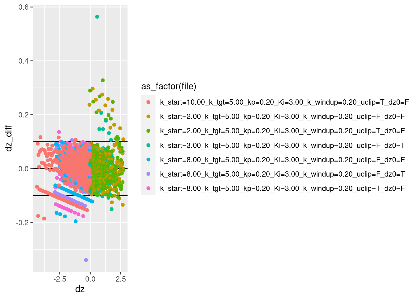

Past versions of unnamed-chunk-9-1.png

Version	Author	Date
867778a	Ross Gayler	2021-08-11

• Most of the estimated velocities are within the calculated range of approximation error.

• There are a modest number of points between the calculated errors bound and three times the error bound.

• There are a few points with error more than three times the error bound.

The estimated velocity is likely to have larger estimation errors when the acceleration is high, because the velocity is changing more rapidly. Take a look at velocity estimation error as a function of acceleration.

# velocity_error ~ acceleration
d %>% ggplot() +
  geom_hline(yintercept = c(-0.1, 0, 0.1)) +
  geom_smooth(aes(x = d2z_est, y = dz_diff)) +
  geom_point(aes(x = d2z_est, y = dz_diff, colour = as_factor(file)))

`geom_smooth()` using method = 'gam' and formula 'y ~ s(x, bs = "cs")'

Warning: Removed 7 rows containing non-finite values (stat_smooth).

Warning: Removed 7 rows containing missing values (geom_point).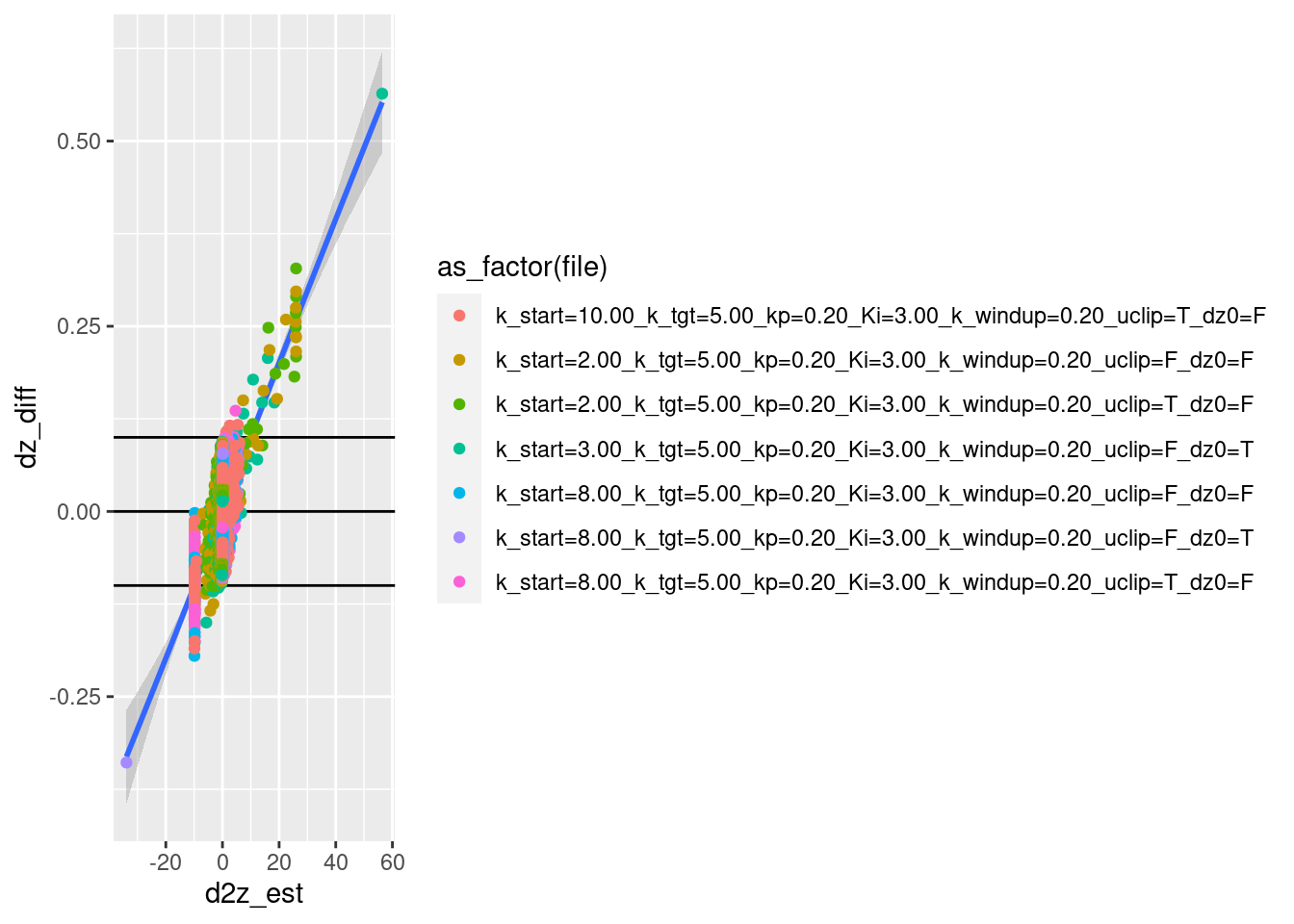

Past versions of unnamed-chunk-10-1.png

Version	Author	Date
867778a	Ross Gayler	2021-08-11

• The estimation error is pretty much explained by the acceleration.

I am happy that the input altitude and velocity are correctly related.

2 Plots

Plot the relationships between the major nodes. This is not necessarily of immediate use in deciding the design fo VSA components, but gives a feel for the dynamics of the system.

2.1 Time explicit

Show the values of the major nodes as a function of time.

2.1.1 Altitude versus time:

p <- d_wide %>% 
  dplyr::mutate(
    k_start = k_start %>% forcats::as_factor(),
    d2z = (dz - lag(dz, n = 1, default = NA)) / 0.010 # get vertical acceleration
  ) %>% 
  ggplot(aes(x = t, group = file, colour = k_start))

p + geom_path(aes(y = z))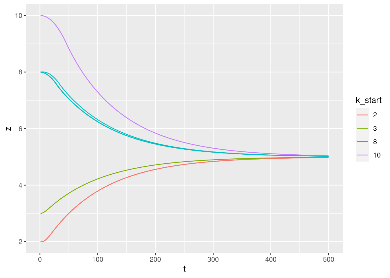

Past versions of unnamed-chunk-11-1.png

Version	Author	Date
867778a	Ross Gayler	2021-08-11

Altitude versus time:

• Looks clean and reasonable.

2.1.2 Velocity versus time:

p + geom_path(aes(y = dz))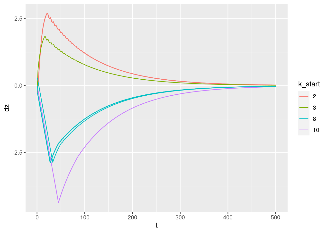

Past versions of unnamed-chunk-12-1.png

Version	Author	Date
867778a	Ross Gayler	2021-08-11

Velocity versus time:

• Looks reasonable, but …
• The sharp peaks in all curves indicate that the controller is initially heading for the target altitude as fast as possible, then suddenly switches into a mode where it tapers off the effort.
• The oscillations visible in the curves for 2 and 3 metre starting height are a bit odd. I suspect they mean that the tuning of the PID controller could be improved.

Zoom in on the oscillation in the \(k_{start} = 2\) curve to see how the oscillation is aligned with the sampling rate.

d_wide %>% 
  dplyr::mutate(
    k_start = k_start %>% forcats::as_factor(),
    d2z = (dz - lag(dz, n = 1, default = NA)) / 0.010 # get vertical acceleration
  ) %>% 
  dplyr::filter(k_start == 2) %>% 
  ggplot(aes(x = t, group = file, colour = k_start)) +
  geom_path(aes(y = dz)) +
  geom_point(aes(y = dz)) +
  coord_cartesian(xlim = c(25, 45), ylim = c(2.0, 2.6))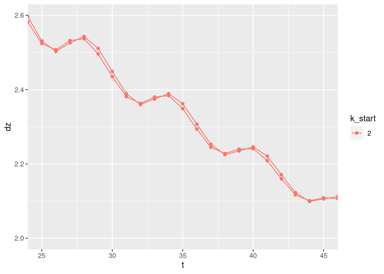

Past versions of unnamed-chunk-13-1.png

Version	Author	Date
867778a	Ross Gayler	2021-08-11

• The cycle length of the oscillation is 6 time steps - so quite rapid, but not the maximum that could be observed (2).

2.1.3 Acceleration versus time

Note that the acceleration should be directly related to the motor power command.

p + geom_path(aes(y = d2z))

Warning: Removed 1 row(s) containing missing values (geom_path).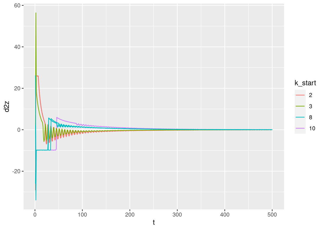

Past versions of unnamed-chunk-14-1.png

Version	Author	Date
867778a	Ross Gayler	2021-08-11

Acceleration versus time:

• The large initial spikes look like they might be artifacts of the estimation of the acceleration (analogous to the estimation errors of the velocity).

Zoom in on the spikes at the start of the curves.

d_wide %>% 
  dplyr::mutate(
    k_start = k_start %>% forcats::as_factor(),
    d2z = (dz - lag(dz, n = 1, default = NA)) / 0.010 # get vertical acceleration
  ) %>% 
  ggplot(aes(x = t, group = file, colour = k_start)) +
  geom_path(aes(y = d2z)) +
  geom_point(aes(y = d2z)) +
  coord_cartesian(xlim = c(1, 20))

Warning: Removed 1 row(s) containing missing values (geom_path).

Warning: Removed 1 rows containing missing values (geom_point).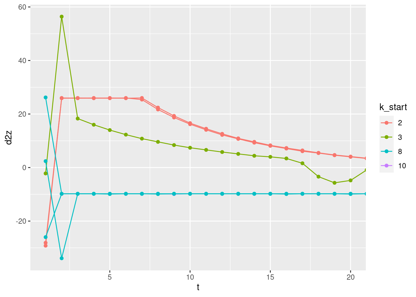

Past versions of unnamed-chunk-15-1.png

Version	Author	Date
867778a	Ross Gayler	2021-08-11

• The acceleration should be maximum and constant when the motor command is 0 or 1. This corresponds to the flat initial segments for starting altitude 2 or 8 metres (10 metres is not visible because of overplotting).

  • The curves for starting altitude above the target have an initial acceleration of approximately \(-10 ms^{-2}\) which is near enough to gravitational acceleration of \(-9.8 ms^{-2}\), considering it is being read off a graph. For the simulations with starting altitude above the target the multicopter initially drops with the motors turned off, so we would expect the initial acceleration to match gravitational acceleration.
  • The curves for starting altitude 2m (well below the 5m target) have an initial acceleration of approximately \(+26 ms^{-2}\). For the simulations with starting altitude 2m the multicopter initially runs the motors at maximum power. The magnitude of the upward acceleration at maximum power relative to the downward acceleration when the motors are off implies that the maximum thrust is 3.6 times the weight of the multicopter. This seems reasonable.

• The acceleration curves look reasonable from time \(t = 3\) onwards.

• There are no issues with the estimated acceleration when the the target altitude changes in the middle of the simulation.

• I conclude that the estimated acceleration is not trustworthy for \(t < 3\).

Re-plot the acceleration curve making the estimated acceleration missing when \(t < 3\).

p <- d_wide %>% 
  dplyr::mutate(
    k_start = k_start %>% forcats::as_factor(),
    d2z = (dz - lag(dz, n = 1, default = NA)) / 0.010, # get vertical acceleration
    d2z = if_else(t >= 3, d2z, NA_real_)
  ) %>% 
  ggplot(aes(x = t, group = file, colour = file))

p + geom_path(aes(y = d2z))

Warning: Removed 14 row(s) containing missing values (geom_path).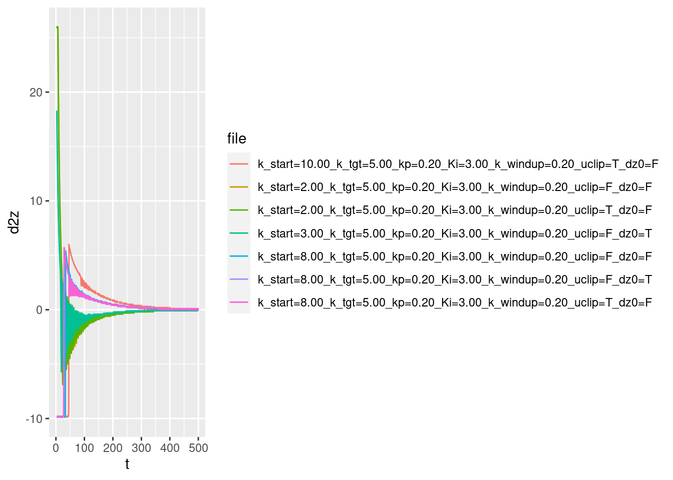

Past versions of unnamed-chunk-16-1.png

Version	Author	Date
867778a	Ross Gayler	2021-08-11

• The oscillations are much more visible.
• It is clear that the oscillations “switch on” at a time that varies by starting height. We’ll see later that the oscillation turns on when the integrated error term (\(ei\)) is not being clipped.
• The oscillations in acceleration imply oscillations in the motor power level.

2.1.4 Error versus time

p + geom_path(aes(y = e))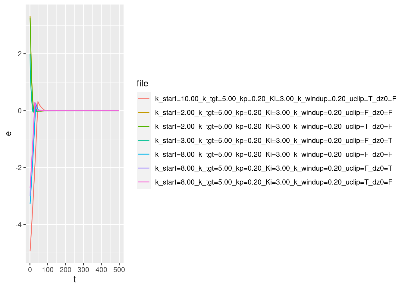

Past versions of unnamed-chunk-17-1.png

Version	Author	Date
867778a	Ross Gayler	2021-08-11

Error versus time:

• The error terms approach zero very rapidly. They are at approximately zero long before the multicopter reaches target height. This is because the error term includes a velocity component, so the error should be interpreted as the predicted error in altitude one second in the future, assuming that the current velocity is maintained for that period.
• Each curve appears to rapidly approach zero then oscillate around zero.
• Each curve appears to eventually settle to zero.

Zoom in on the heads of the curves to see if they really oscillate around zero.

p + 
  geom_hline(yintercept = 0) +
  geom_path(aes(y = e)) +
  geom_point(aes(y = e)) +
  coord_cartesian(xlim = c(10, 100), ylim = c(-0.2, 0.4))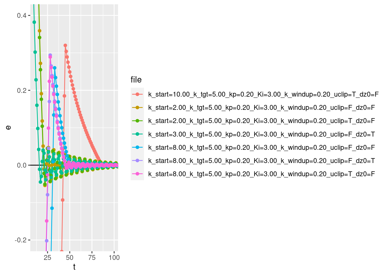

Past versions of unnamed-chunk-18-1.png

Version	Author	Date
867778a	Ross Gayler	2021-08-11

• The error curves oscillate around zero.

Zoom in on the tails of the curves to see how close the error term approaches zero.

p + 
  geom_hline(yintercept = 0) +
  geom_path(aes(y = e)) +
  geom_point(aes(y = e)) +
  coord_cartesian(xlim = c(100, 250), ylim = c(-0.003, 0.003))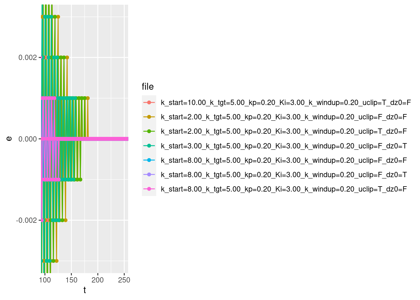

Past versions of unnamed-chunk-19-1.png

Version	Author	Date
867778a	Ross Gayler	2021-08-11

• The error term gets very close to zero. All the curves have reached zero to within the 3 decimal place precision of the import files.

2.1.5 Integrated error versus time

p + geom_path(aes(y = ei))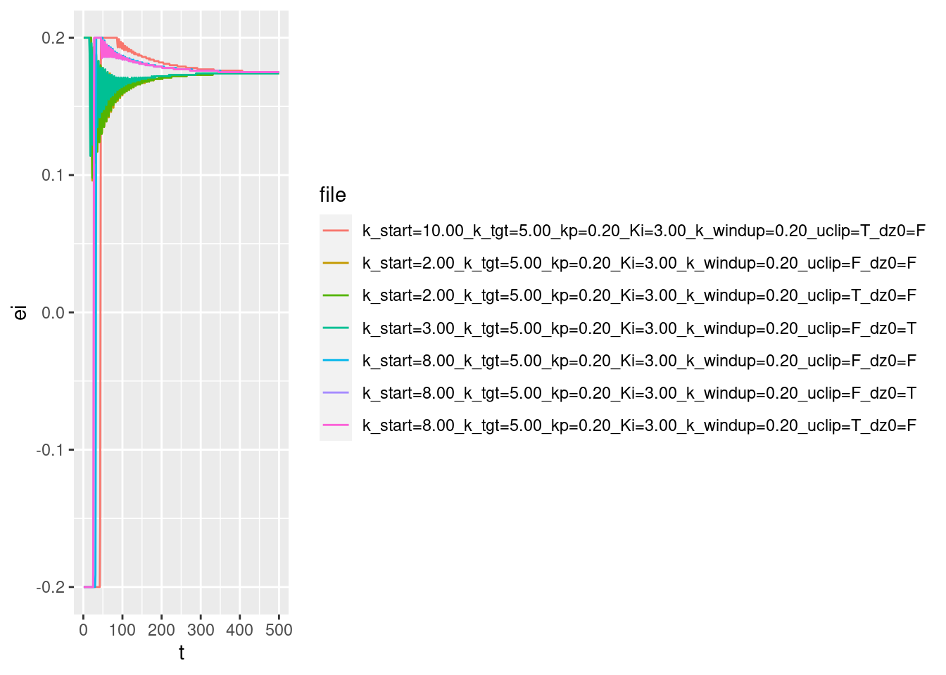

Past versions of unnamed-chunk-20-1.png

Version	Author	Date
867778a	Ross Gayler	2021-08-11

Integrated error versus time:

• The values are bounded between the clipping limits.
• Some early values jump between the negative and positive clipping limits very rapidly.
• Once the curves move into the unclipped value range they oscillate.
• All the curves converge to a value of approximately 0.175. Presumably, this corresponds to the motor power level required for the multicopter to have zero vertical velocity (hover).

2.1.6 Motor command versus time

p + geom_path(aes(y = u))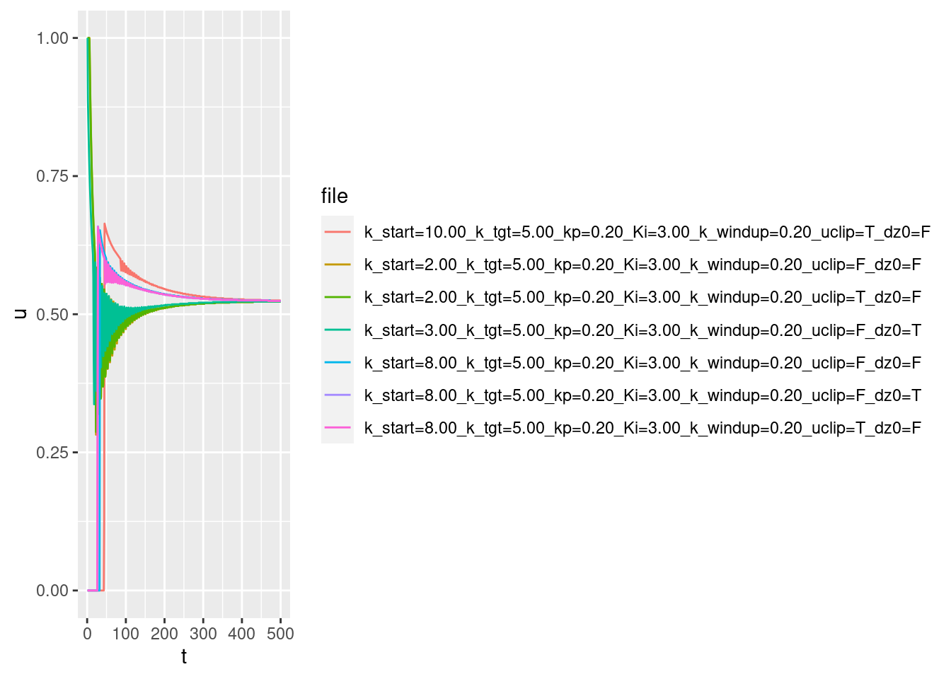

Past versions of unnamed-chunk-21-1.png

Version	Author	Date
867778a	Ross Gayler	2021-08-11

Motor command versus time:

• Curves starting below the target altitude have maximum initial motor command.
• Curves starting above the target altitude have maximum initial motor command.
• All curves show oscillatory behaviour after the initial period of extreme command.
• All curves converge to a value of 0.524. Presumably, this corresponds to the motor power level required for the multicopter to have zero vertical velocity (hover).

2.2 Time implicit

Show the values of the major nodes (\(z\), \(dz\), \(e\), \(ei\), and \(u\), augmented with estimated acceleration: \(d2z\)) as a function of each other (pair plots) with time implicit. There’s no commentary on these graphs - just enjoy the pretty pictures.

Start the curves at time \(t = 3\) to avoid the artifacts in the estimated acceleration seen in first two time steps.

Place an arrow head on each curve to indicate the direction of time. Because the curves tend to converge on the same location I have placed the arrow head at the beginning of each curve (\(t = 3\)). The arrow head points in the direction of increasing time.

p <- d_wide %>% 
  dplyr::mutate(
    k_start = k_start %>% forcats::as_factor(),
    d2z = (dz - lag(dz, n = 1, default = NA)) / 0.010  # get vertical acceleration
  ) %>% 
  dplyr::filter(t >= 3) %>% 
  ggplot(aes(group = file, colour = k_start))

a <- grid::arrow(ends = "first", angle = 150, type = "closed")

###

p + geom_vline(xintercept = 5) + geom_hline(yintercept = 0) +
  geom_path(aes(x = z, y = dz), arrow = a, alpha = 0.2) + 
  geom_point(aes(x = z, y = dz), size = 0.1)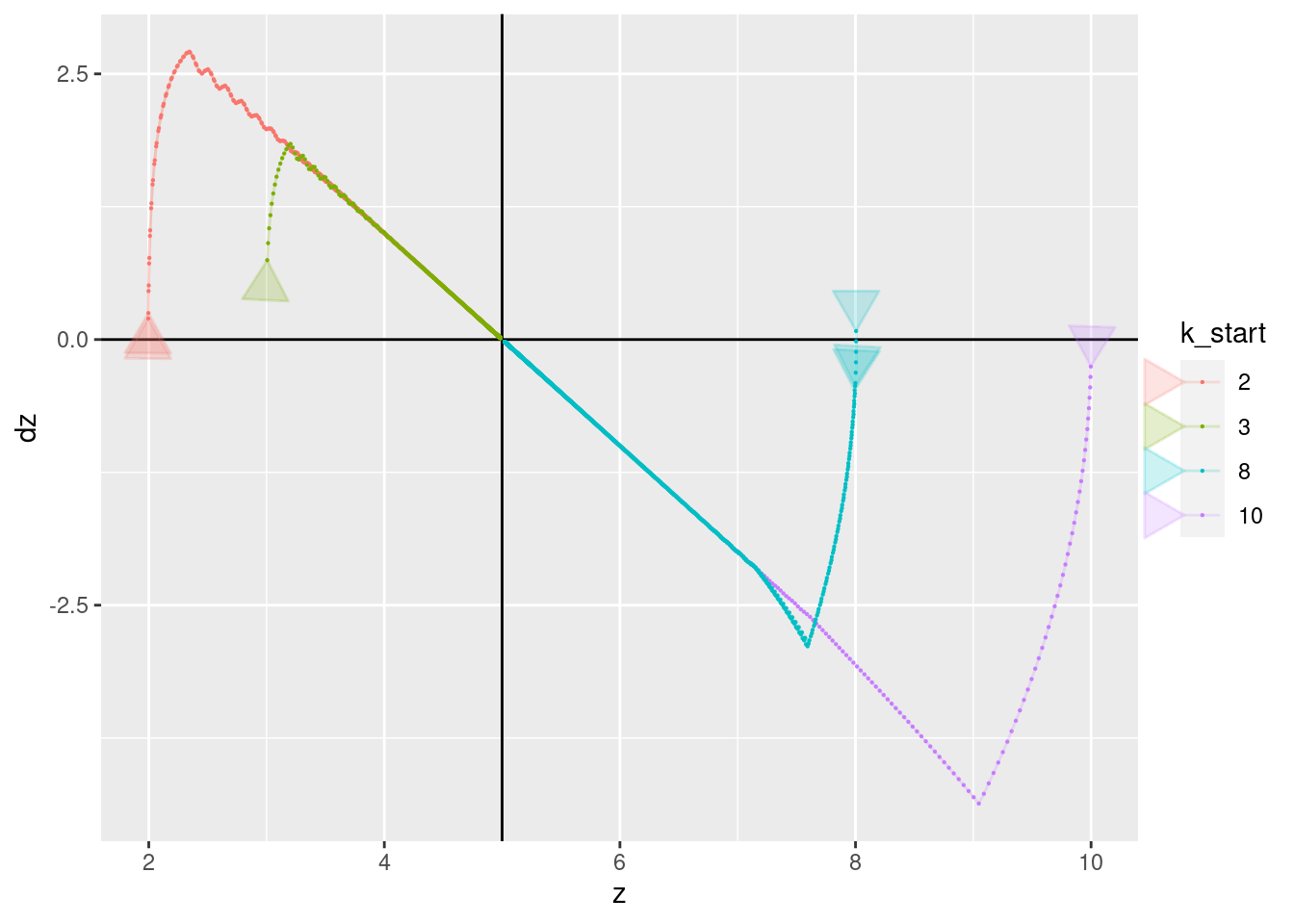

Past versions of unnamed-chunk-22-1.png

Version	Author	Date
867778a	Ross Gayler	2021-08-11

p + geom_vline(xintercept = 5) + geom_hline(yintercept = 0) +
  geom_path(aes(x = z, y = d2z), arrow = a, alpha = 0.2) + 
  geom_point(aes(x = z, y = d2z), size = 0.1)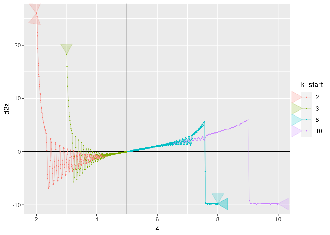

Past versions of unnamed-chunk-22-2.png

Version	Author	Date
867778a	Ross Gayler	2021-08-11

p + geom_vline(xintercept = 5) + geom_hline(yintercept = 0) +
  geom_path(aes(x = z, y = e), arrow = a, alpha = 0.2) + 
  geom_point(aes(x = z, y = e), size = 0.1)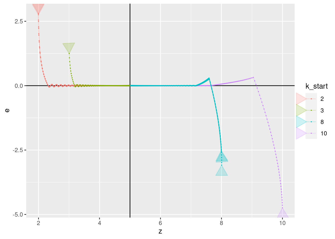

Past versions of unnamed-chunk-22-3.png

Version	Author	Date
867778a	Ross Gayler	2021-08-11

p + geom_vline(xintercept = 5) + geom_hline(yintercept = 0.175) +
  geom_path(aes(x = z, y = ei), arrow = a, alpha = 0.2) + 
  geom_point(aes(x = z, y = ei), size = 0.1)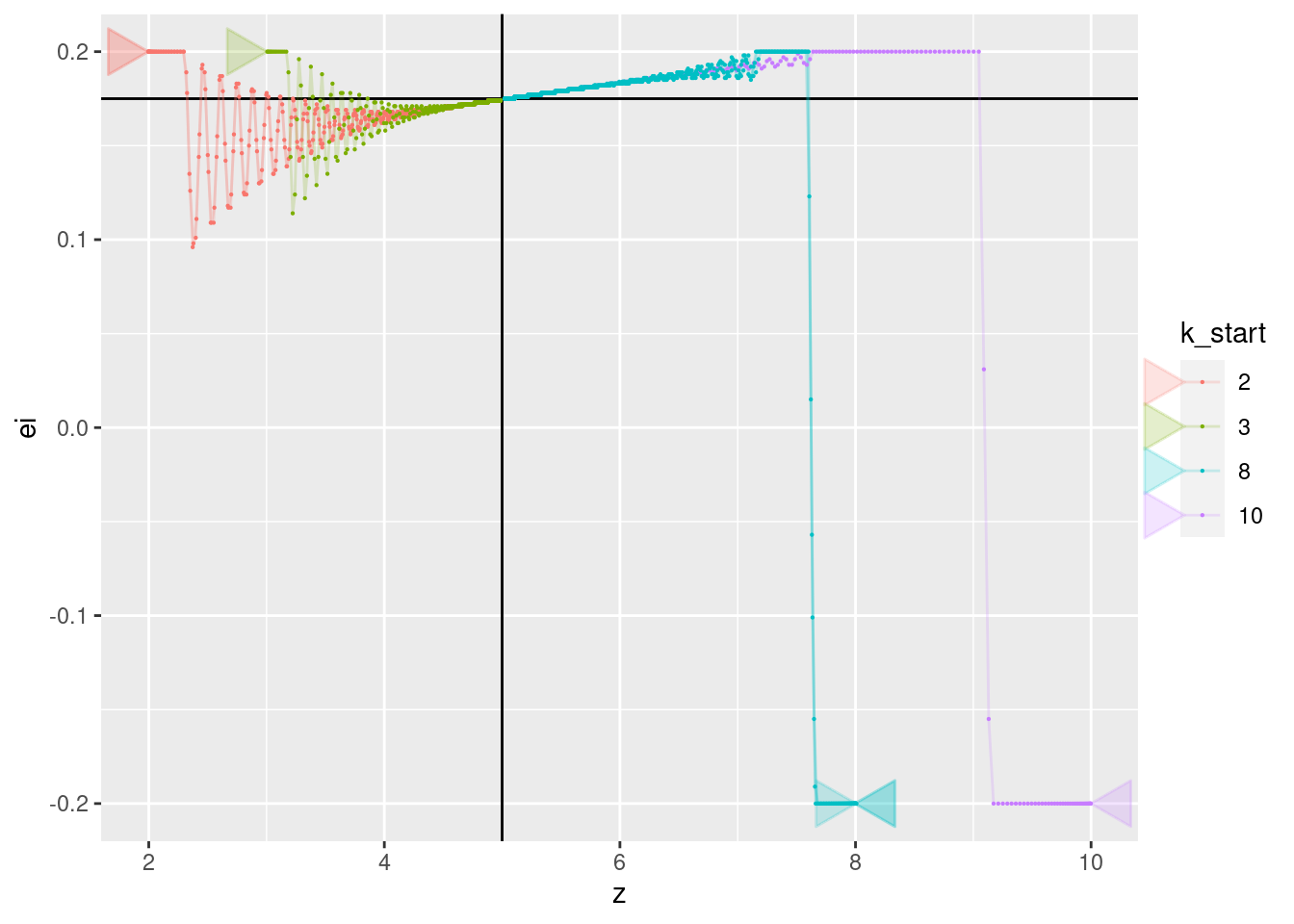

Past versions of unnamed-chunk-22-4.png

Version	Author	Date
867778a	Ross Gayler	2021-08-11

p + geom_vline(xintercept = 5) + geom_hline(yintercept = 0.524) +
  geom_path(aes(x = z, y = u), arrow = a, alpha = 0.2) + 
  geom_point(aes(x = z, y = u), size = 0.1)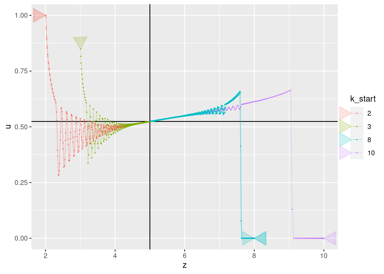

Past versions of unnamed-chunk-22-5.png

Version	Author	Date
867778a	Ross Gayler	2021-08-11

###

p + geom_vline(xintercept = 0) + geom_hline(yintercept = 0) +
  geom_path(aes(x = dz, y = d2z), arrow = a, alpha = 0.2) + 
  geom_point(aes(x = dz, y = d2z), size = 0.1)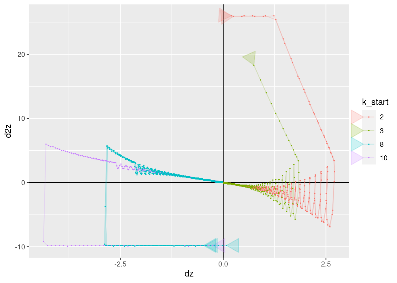

Past versions of unnamed-chunk-22-6.png

Version	Author	Date
867778a	Ross Gayler	2021-08-11

p + geom_vline(xintercept = 0) + geom_hline(yintercept = 0) +
  geom_path(aes(x = dz, y = e), arrow = a, alpha = 0.2) + 
  geom_point(aes(x = dz, y = e), size = 0.1)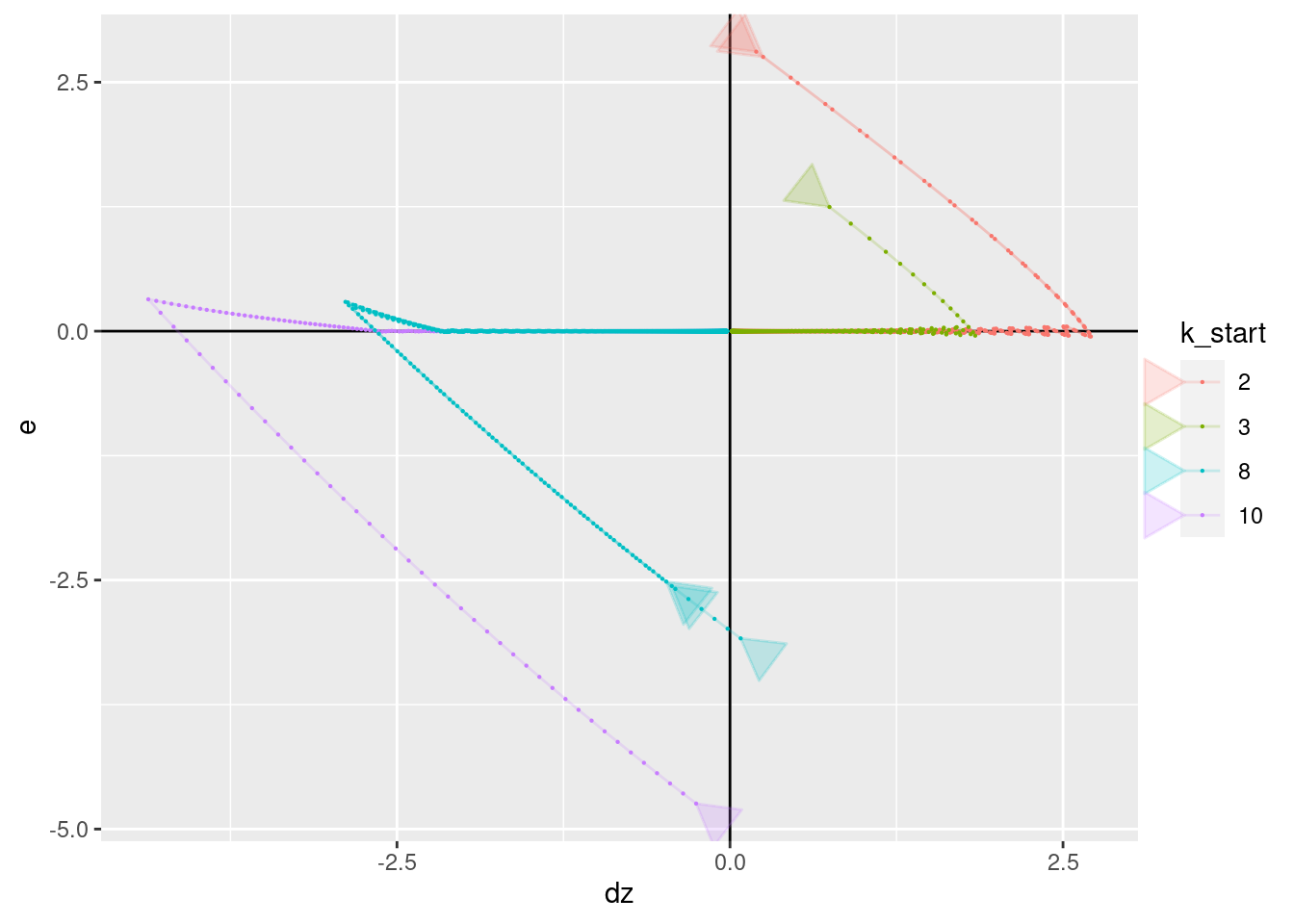

Past versions of unnamed-chunk-22-7.png

Version	Author	Date
867778a	Ross Gayler	2021-08-11

p + geom_vline(xintercept = 0) + geom_hline(yintercept = 0.175) +
  geom_path(aes(x = dz, y = ei), arrow = a, alpha = 0.2) + 
  geom_point(aes(x = dz, y = ei), size = 0.1)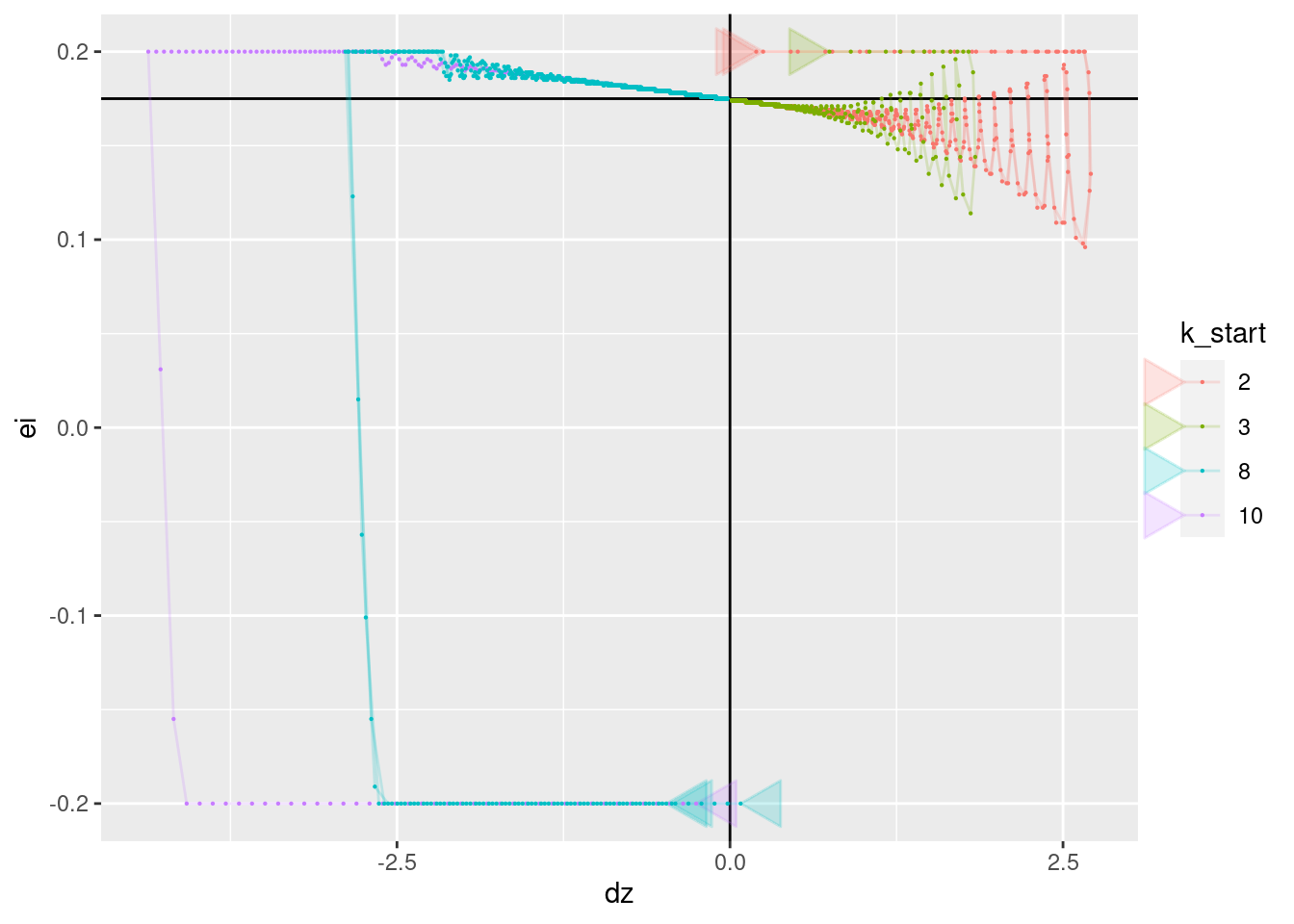

Past versions of unnamed-chunk-22-8.png

Version	Author	Date
867778a	Ross Gayler	2021-08-11

p + geom_vline(xintercept = 0) + geom_hline(yintercept = 0.524) +
  geom_path(aes(x = dz, y = u), arrow = a, alpha = 0.2) + 
  geom_point(aes(x = dz, y = u), size = 0.1)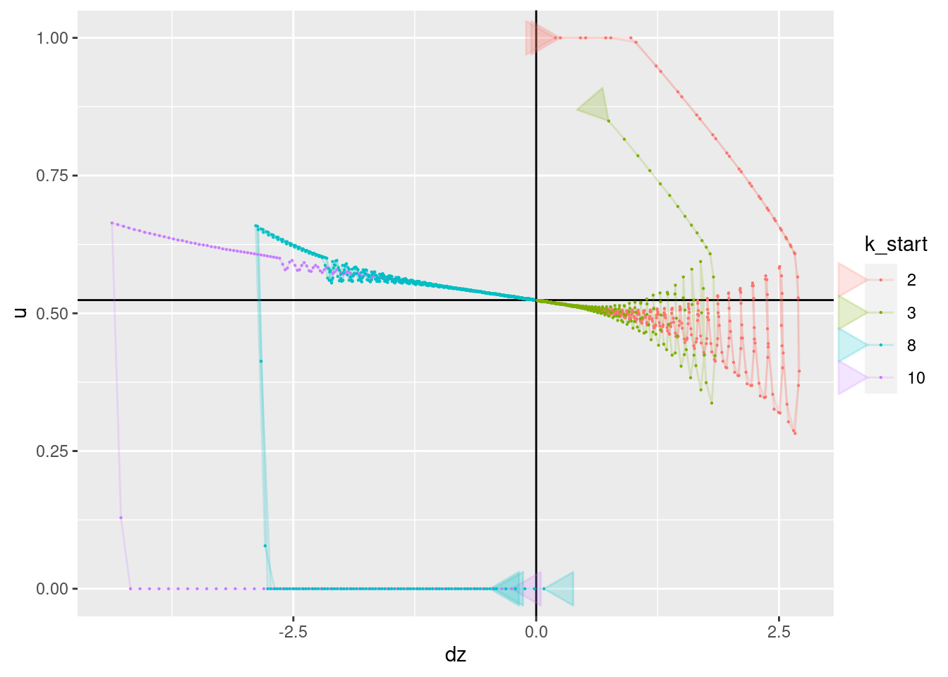

Past versions of unnamed-chunk-22-9.png

Version	Author	Date
867778a	Ross Gayler	2021-08-11

###

p + geom_vline(xintercept = 0) + geom_hline(yintercept = 0) +
  geom_path(aes(x = d2z, y = e), arrow = a, alpha = 0.2) + 
  geom_point(aes(x = d2z, y = e), size = 0.1)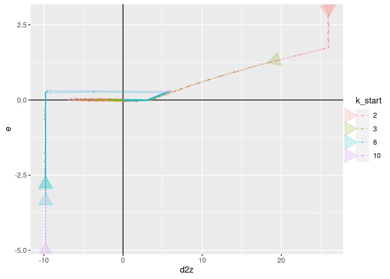

Past versions of unnamed-chunk-22-10.png

Version	Author	Date
867778a	Ross Gayler	2021-08-11

p + geom_vline(xintercept = 0) + geom_hline(yintercept = 0.175) +
  geom_path(aes(x = d2z, y = ei), arrow = a, alpha = 0.2) + 
  geom_point(aes(x = d2z, y = ei), size = 0.1)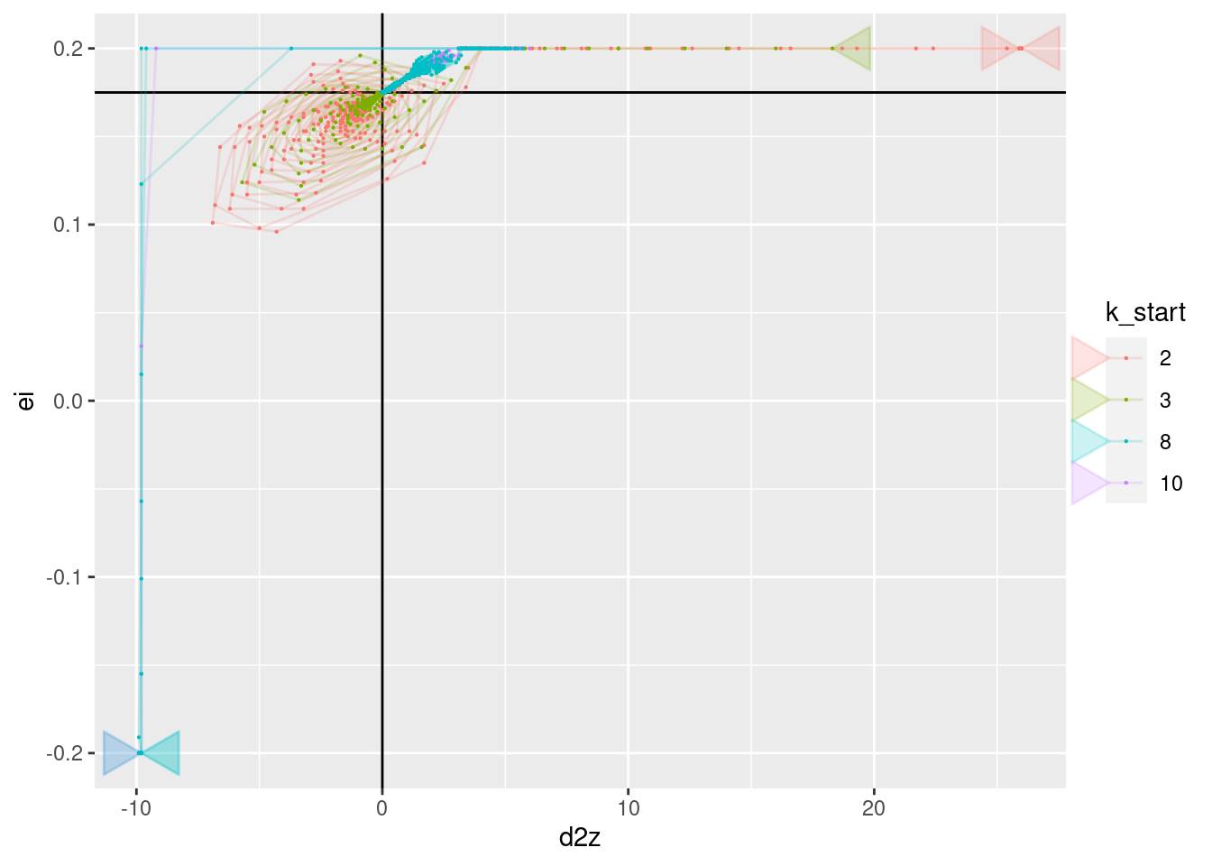

Past versions of unnamed-chunk-22-11.png

Version	Author	Date
867778a	Ross Gayler	2021-08-11

p + geom_vline(xintercept = 0) + geom_hline(yintercept = 0.524) +
  geom_path(aes(x = d2z, y = u), arrow = a, alpha = 0.2) + 
  geom_point(aes(x = d2z, y = u), size = 0.1)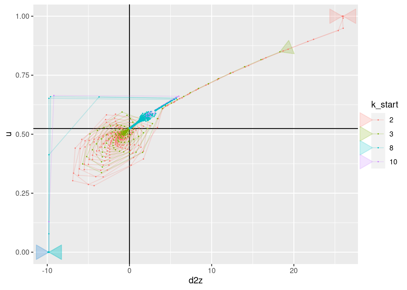

Past versions of unnamed-chunk-22-12.png

Version	Author	Date
867778a	Ross Gayler	2021-08-11

###

p + geom_vline(xintercept = 0) + geom_hline(yintercept = 0.175) +
  geom_path(aes(x = e, y = ei), arrow = a, alpha = 0.2) + 
  geom_point(aes(x = e, y = ei), size = 0.1)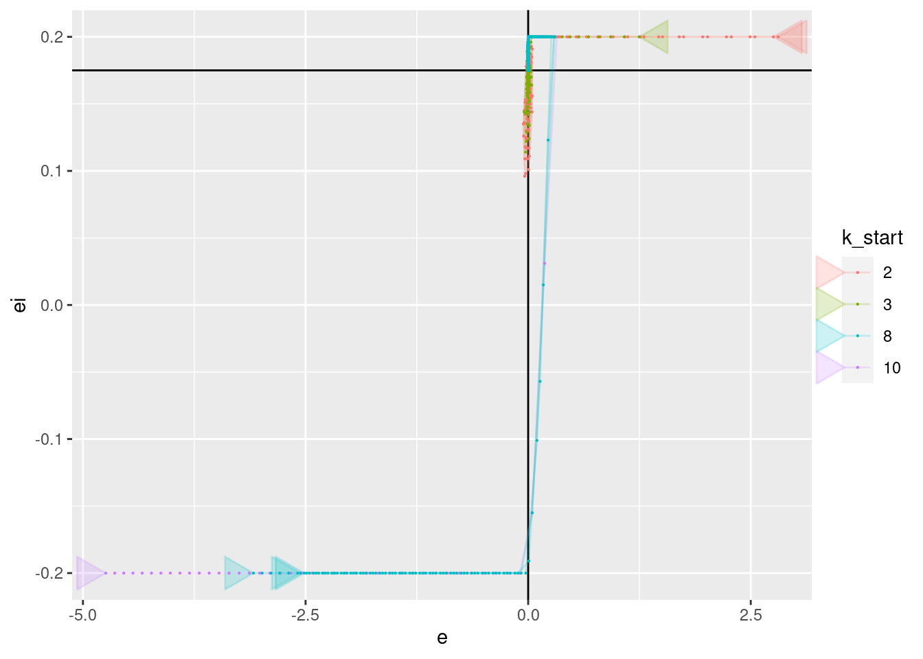

Past versions of unnamed-chunk-22-13.png

Version	Author	Date
867778a	Ross Gayler	2021-08-11

p + geom_vline(xintercept = 0) + geom_hline(yintercept = 0.524) +
  geom_path(aes(x = e, y = u), arrow = a, alpha = 0.2) + 
  geom_point(aes(x = e, y = u), size = 0.1)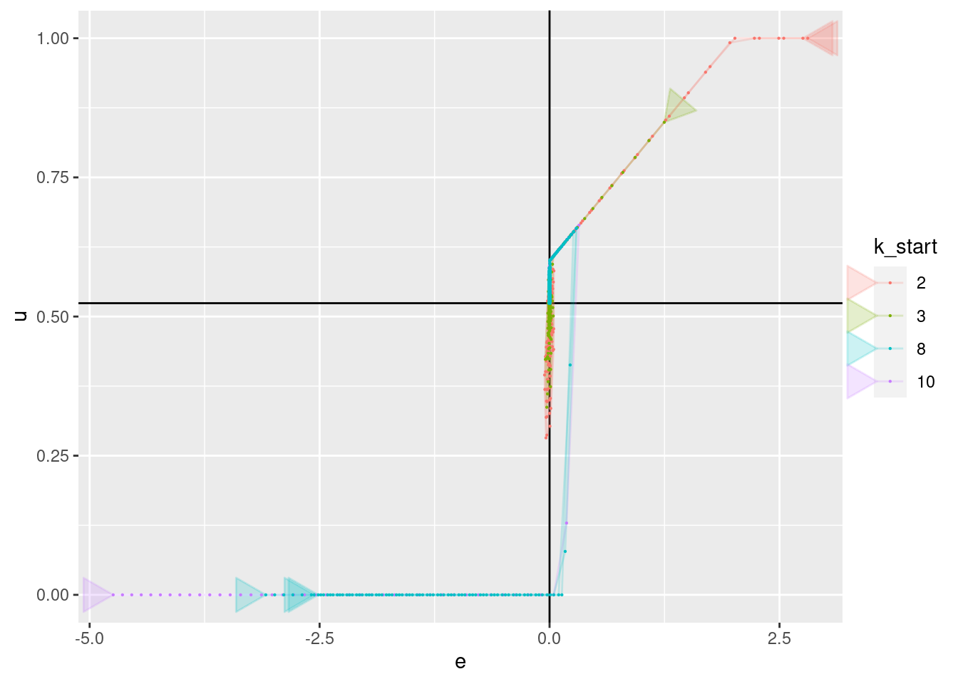

Past versions of unnamed-chunk-22-14.png

Version	Author	Date
867778a	Ross Gayler	2021-08-11

###

p + geom_vline(xintercept = 0.175) + geom_hline(yintercept = 0.524) +
  geom_path(aes(x = ei, y = u), arrow = a, alpha = 0.2) + 
  geom_point(aes(x = ei, y = u), size = 0.1)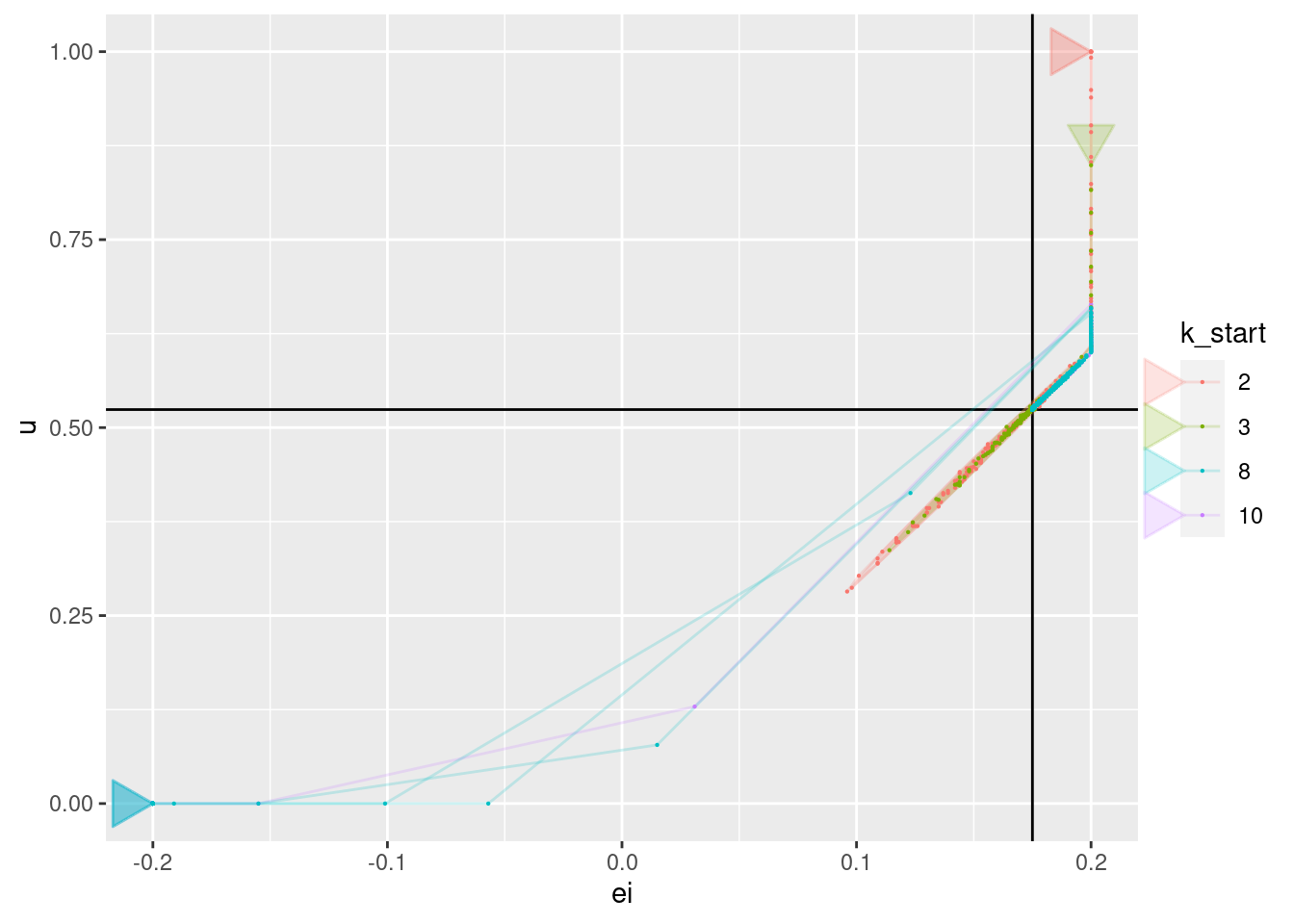

Past versions of unnamed-chunk-22-15.png

Version	Author	Date
867778a	Ross Gayler	2021-08-11

3 Distributions

Look at the distributions of the values of all the nodes of the data flow diagram.

Note that these distributions are calculated over all the input files pooled.

Also note that the concept of a distribution is somewhat suspect when applied to an arbitrary selection of nonstationary signals.

3.1 Summary dsitributions

Display a quick summary of the distributions of values of all the nodes (except the parameter nodes) and those internal nodes which are identical to imported nodes (\(i2 := e\), \(i5 := ei\), and \(i8 := u\)).

The observed minimum (\(p0\)) and maximum (\(p100\)) will inform the value ranges of the corresponding VSA representations.

d_wide %>% 
  dplyr::select(z:u, i1, i3, i4, i6, i7) %>% 
  skimr::skim()

Table 3.1: Data summary

Name	Piped data
Number of rows	3500
Number of columns	10
_______________________
Column type frequency:
numeric	10
________________________
Group variables	None

Variable type: numeric

skim_variable	n_missing	complete_rate	mean	sd	p0	p25	p50	p75	p100	hist
z	0	1	5.22	1.15	2.00	4.85	5.05	5.44	10.00	▁▇▃▁▁
dz	0	1	-0.17	0.98	-4.37	-0.43	-0.05	0.15	2.71	▁▁▅▇▁
e	0	1	-0.05	0.46	-4.94	0.00	0.00	0.00	3.32	▁▁▇▁▁
ei	0	1	0.16	0.07	-0.20	0.17	0.17	0.18	0.20	▁▁▁▁▇
u	0	1	0.51	0.11	0.00	0.52	0.52	0.53	1.00	▁▁▇▁▁
i1	0	1	-0.22	1.15	-5.00	-0.44	-0.05	0.15	3.00	▁▁▃▇▁
i3	0	1	-0.01	0.09	-0.99	0.00	0.00	0.00	0.66	▁▁▇▁▁
i4	0	1	0.12	0.52	-5.04	0.17	0.17	0.18	3.50	▁▁▁▇▁
i6	0	1	0.49	0.21	-0.60	0.52	0.52	0.53	0.60	▁▁▁▁▇
i7	0	1	0.48	0.29	-1.59	0.52	0.52	0.53	1.26	▁▁▁▇▁

3.2 Detailed distributions

Look at the detailed distribution of all the nodes (except the parameter nodes) and those internal nodes which are identical to imported nodes (\(i2 := e\), \(i5 := ei\), and \(i8 := u\)).

The distributions will give some idea about how much different regions of the value ranges are used.

Use a logarithmic scale for the counts to bring out the detail in the low density areas.

Also, divide the ranges into quintiles to give an idea of where range boundaries might be if we used a low resolution representation (effectively dividing each value range into “high negative”, “medium negative”, “neutral”, “medium positive”, “high positive”). This is relevant to the question of value resolution.

d_node <- d_wide %>% 
  dplyr::select(z:u, i1, i3, i4, i6, i7) %>% 
  tidyr::pivot_longer(cols = everything(), names_to = "node", values_to = "value")

d_quintile <- d_node %>%  
  dplyr::group_by(node) %>% 
  dplyr::summarise(
    p01 = quantile(value, probs = 0.01, names = FALSE),
    p02 = quantile(value, probs = 0.02, names = FALSE),
    p05 = quantile(value, probs = 0.05, names = FALSE),
    p20 = quantile(value, probs = 0.2, names = FALSE),
    p40 = quantile(value, probs = 0.4, names = FALSE),
    p60 = quantile(value, probs = 0.6, names = FALSE),
    p80 = quantile(value, probs = 0.8, names = FALSE),
    p95 = quantile(value, probs = 0.95, names = FALSE),
    p98 = quantile(value, probs = 0.98, names = FALSE),
    p99 = quantile(value, probs = 0.99, names = FALSE)
  )

d_node %>% 
  ggplot(aes(x = value)) +
  facet_wrap(facets = vars(node), ncol = 2, scales = "free") +
  geom_histogram(bins = 50) +
  scale_y_log10() +
  geom_vline(data = d_quintile, aes(xintercept = p01), colour = "orange", linetype = "dotted") +
  geom_vline(data = d_quintile, aes(xintercept = p02), colour = "orange", linetype = "dashed") +
  geom_vline(data = d_quintile, aes(xintercept = p05), colour = "orange", linetype = "solid") +
  geom_vline(data = d_quintile, aes(xintercept = p20), colour = "red", linetype = "dashed") +
  geom_vline(data = d_quintile, aes(xintercept = p40), colour = "red", linetype = "solid") +
  geom_vline(data = d_quintile, aes(xintercept = p60), colour = "red", linetype = "solid") +
  geom_vline(data = d_quintile, aes(xintercept = p80), colour = "red", linetype = "dashed") +
  geom_vline(data = d_quintile, aes(xintercept = p95), colour = "orange", linetype = "solid") +
  geom_vline(data = d_quintile, aes(xintercept = p98), colour = "orange", linetype = "dashed") +
  geom_vline(data = d_quintile, aes(xintercept = p99), colour = "orange", linetype = "dotted")

Warning: Transformation introduced infinite values in continuous y-axis

Warning: Removed 84 rows containing missing values (geom_bar).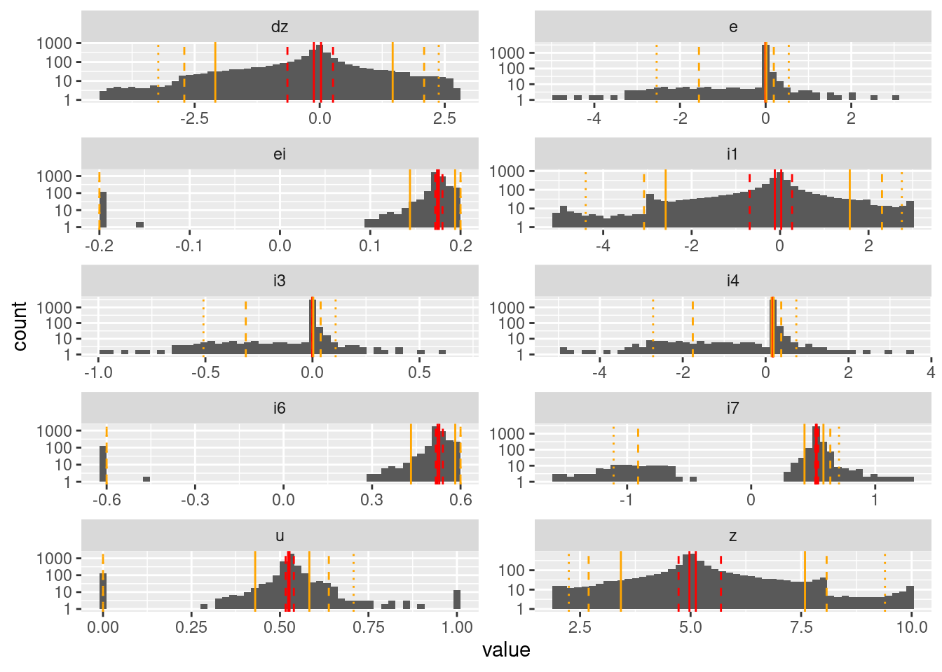

Past versions of unnamed-chunk-24-1.png

Version	Author	Date
867778a	Ross Gayler	2021-08-11

• Values which are driven to a target (\(z\), \(i1\), \(dz\), \(e\), \(i3\)) have unimodal distributions.

• Values driven by the integrated error (\(ei\), \(i6\), \(i7\)) have bimodal distributions.

  • \(i4\) is part of the calculation of integrated error, but is dominated by \(e\), so has a unimodal distribution.

• The values of motor command (\(u\)) have a trimodal distribution (full on, full off, hovering).

• The quintiles are very closely clustered around the principal mode of each distribution. This indicates that a quintile-based resolution would not be very useful.

  • This suggests that an encoding would either need to be based on the values rather than quantiles, or quantiles would have to be defined with respect to when the system dynamics is doing something interesting.

4 Value resolution

VSA representations, like any physical implementation have limited value resolution. In this section I would like find the value resolution that is required by the PID controller in order to work satisfactorily. I won’t be doing that because that is probably more effort than is justified at this stage. A proper answer to that question would probably involve something like injecting noise into the value at each node to see how PID performance decreases as noise is increased.

Instead, I will try to get some feel for the effective value resolution in the classically implemented PID controller. I will do this by looking at the distribution of the differences between successive values. The intuition behind this is that the differences between successive values represent the increments in which the state of the dynamic system evolves.

This analysis will not provide any conclusive answers. Rather, it will provide some context for later thinking about the VSA designs.

I expect that the initial VSA designs will be thoroughly over-resourced, so that they have far more value resolution than is required for implementation of the PID controller.

Look at the distributions of absolute differences of successive values at each node.

Exclude observations where the successive difference is zero, because eventually all node values will converge to a steady state which is uninteresting and can be arbitrarily prolonged.

# function to calculate the absolute successive difference
abs_diff <- function(
  x # numeric - vector of values at successive time steps
) # value # numeric - vector of absolute values of first differences
{
  (x - dplyr::lag(x)) %>% abs()
}

d_node <- d_wide %>% 
  dplyr::select(file, t, z:u, i1, i3, i4, i6, i7) %>% 
  dplyr::arrange(file, t) %>% # guarantee correct order for successive differences
  dplyr::group_by(file) %>% 
  dplyr::mutate(
    across(z:i7, abs_diff)
  ) %>% 
  dplyr::ungroup() %>% 
  dplyr::select(-file, -t) %>% 
  tidyr::pivot_longer(cols = everything(), names_to = "node", values_to = "value") %>% 
  dplyr::filter(!is.na(value) & value > 0) # exclude rows with zero change

# calculate quantiles for each node
d_quintile <- d_node %>%  
  dplyr::group_by(node) %>% 
  dplyr::summarise(
    p01 = quantile(value, probs = 0.01, names = FALSE),
    p02 = quantile(value, probs = 0.02, names = FALSE),
    p05 = quantile(value, probs = 0.05, names = FALSE),
    p20 = quantile(value, probs = 0.2, names = FALSE),
    p40 = quantile(value, probs = 0.4, names = FALSE),
    p60 = quantile(value, probs = 0.6, names = FALSE),
    p80 = quantile(value, probs = 0.8, names = FALSE),
    p95 = quantile(value, probs = 0.95, names = FALSE),
    p98 = quantile(value, probs = 0.98, names = FALSE),
    p99 = quantile(value, probs = 0.99, names = FALSE)
  )

d_node %>% 
  ggplot(aes(x = value)) +
  facet_wrap(facets = vars(node), ncol = 2, scales = "free") +
  geom_histogram(bins = 50) +
  scale_x_log10() +
  scale_y_log10() +
  geom_vline(data = d_quintile, aes(xintercept = p01), colour = "orange", linetype = "dotted") +
  geom_vline(data = d_quintile, aes(xintercept = p02), colour = "orange", linetype = "dashed") +
  geom_vline(data = d_quintile, aes(xintercept = p05), colour = "orange", linetype = "solid") +
  geom_vline(data = d_quintile, aes(xintercept = p20), colour = "red", linetype = "dashed") +
  geom_vline(data = d_quintile, aes(xintercept = p40), colour = "red", linetype = "solid") +
  geom_vline(data = d_quintile, aes(xintercept = p60), colour = "red", linetype = "solid") +
  geom_vline(data = d_quintile, aes(xintercept = p80), colour = "red", linetype = "dashed") +
  geom_vline(data = d_quintile, aes(xintercept = p95), colour = "orange", linetype = "solid") +
  geom_vline(data = d_quintile, aes(xintercept = p98), colour = "orange", linetype = "dashed") +
  geom_vline(data = d_quintile, aes(xintercept = p99), colour = "orange", linetype = "dotted")

Warning: Transformation introduced infinite values in continuous y-axis

Warning: Removed 149 rows containing missing values (geom_bar).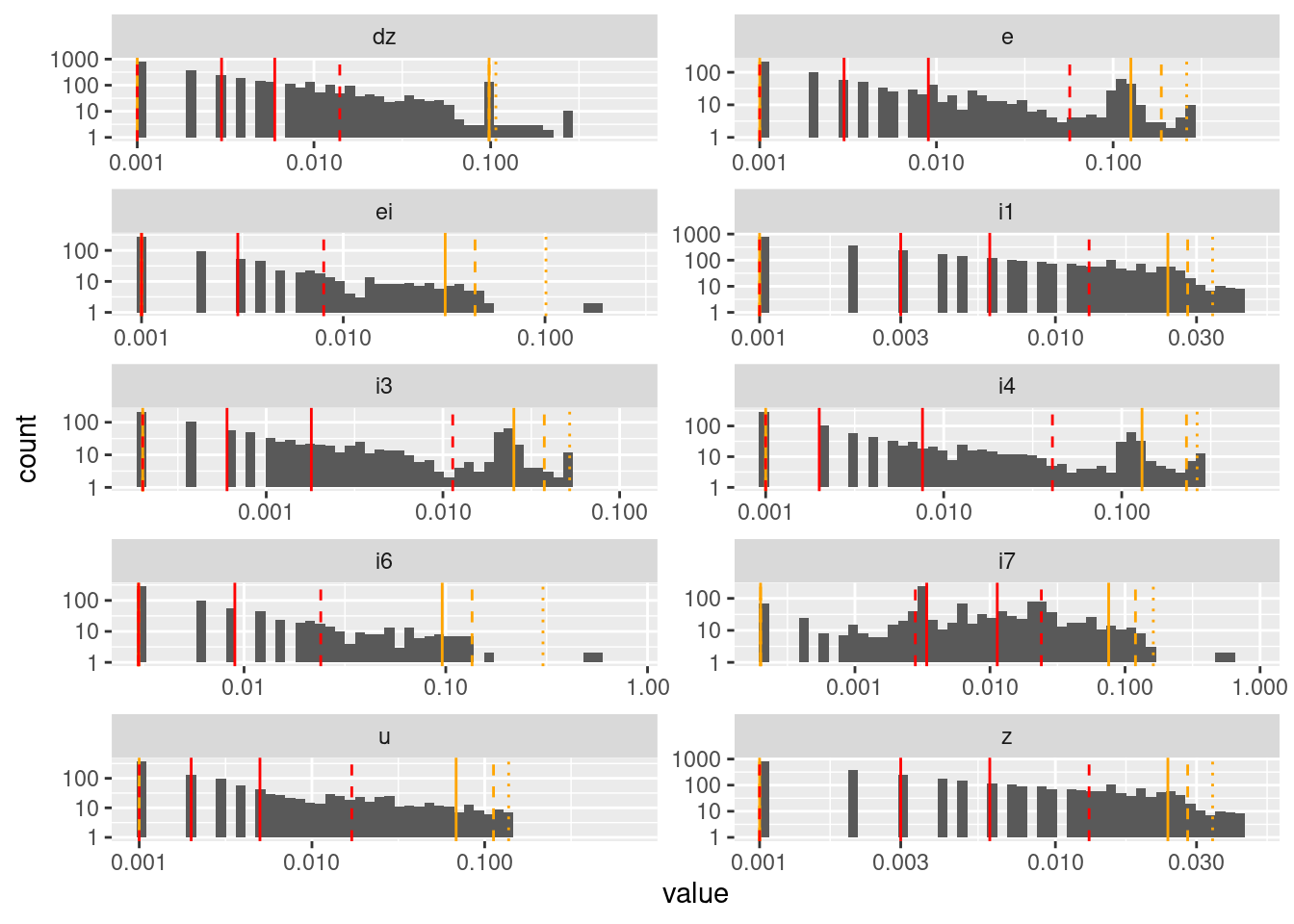

Past versions of unnamed-chunk-25-1.png

Version	Author	Date
867778a	Ross Gayler	2021-08-11

• The pattern of separated bars is due to the values being quantised to three decimal places.

• Successive differences are very heavily concentrated near zero for all nodes.

• Some nodes (\(dz\), \(e\), \(i3\), \(i4\)) have a secondary mode that is clearly nonzero.

• Node \(i7\) has a possibly bimodal distribution.

I don’t know that I would draw any conclusions from that analysis, other than that most values evolve in small increments, and when the increments are large it is probably in the initial stages of detecting and reacting to a large mismatch to the target.

5 Temporal resolution

Temporal resolution is possibly even more problematic than value resolution.

I will look at the power spectra of the values. The data being analysed here is generated by the classically implemented simulation. So the frequencies with relatively higher power will be interpreted as important to the dynamics of the classically implemented PID controller.

Looking at the earlier plots of values as a function of time, I would expect the low frequencies to be prominent as many of the curves show a slow and smooth approach to a target value.

However, there will be some high frequency components corresponding to the sudden turning on or off of the motors.

I also expect to see some frequency component corresponding to the observed oscillatory behaviour. However, this might not be essential to the dynamics of the PID as I suspect the oscillation is an undesired behaviour that could be removed by tuning.

I will look at the power spectrum for each node for an episode of settling (i.e. the period from when a target altitude is set until the target altitude changes or the simulation finishes). This averages over the simulation files. This is a slightly odd set to be averaging over because the responses to the different episodes probably don’t constitute a stationary signal, but I am going to take the episodes as being representative of the system’s behaviour.

Some nodes are redundant (they have identical spectra to other nodes) because they are linear transforms of the other nodes. The redundant nodes have been removed from the plots.

• \(i1\) (= \(z\) minus constant)
• \(i3\) (= \(e\) times constant)
• \(i6\) (= \(ei\) times constant)

The ordering of the node plots corresponds to ordering of the nodes along the data flow diagram from altitude (\(z\)) to motor command (\(u\)).

The spectra are displayed as functions of period rather than frequency because this makes them a little easier to relate to the dynamics observed in the graphs of node value as a function of time.

Both the period and power axes are displayed on logarithmic scales.

# NEW
# function to spectral analyse one time series as a frame
spec_an <- function(
  d # data frame - contains a "value" column
) # value # spectrum object - result of spectral analysis of d
{
  spec_obj <- d %>% 
    dplyr::pull(value) %>% # get the time series of values
    scale() %>% # centre and standardise the time series
    spectrum(
      method = "pgram", detrend = TRUE, plot = FALSE
    ) # return a spectrum object
  
  tibble(freq = spec_obj[["freq"]], spec = spec_obj[["spec"]])
}

d_wide %>% 
  dplyr::select(file, t, z, dz, e, i4, ei, i7, u) %>% # only keep non-redundant nodes
  dplyr::arrange(file, t) %>% # guarantee correct time order
  tidyr::pivot_longer(cols = z:u, names_to = "node", values_to = "value") %>% 
  tidyr::nest(node_series = c(t, value)) %>%  # analysis per episode x node
  dplyr::mutate(
    spectrum = node_series %>% map(spec_an), # calculate the spectra
    node = node %>% forcats::fct_relevel(
      c("z", "dz", "e", "i4", "ei", "i7", "u")
      ) # reorder levels of node for display
  ) %>% 
  dplyr::select(-node_series) %>% # drop time series
  tidyr::unnest(cols = spectrum) %>%
  dplyr::group_by(node, freq) %>% # average over file
  dplyr::summarise(spec = mean(spec), .groups = "drop") %>%
  ggplot() +
  geom_vline(xintercept = 6, alpha = 0.2) +
  geom_path(aes(x = 1/freq, y = spec)) +
  geom_point(aes(x = 1/freq, y = spec), size = 0.5) +
  scale_x_log10() + scale_y_log10() +
  xlab("Period (time steps)") + ylab("Power") +
  facet_wrap(vars(node), ncol = 4)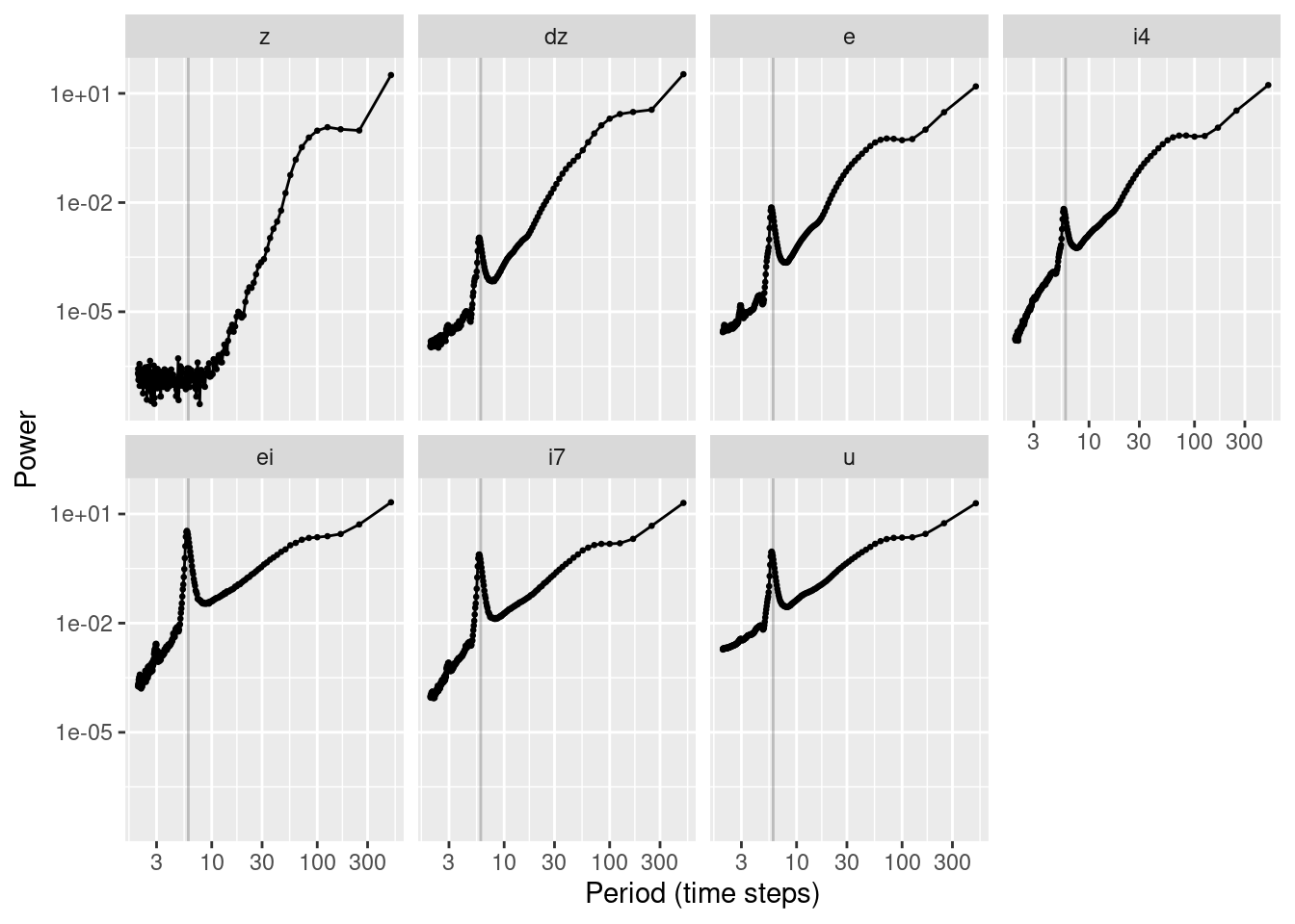

Past versions of unnamed-chunk-26-1.png

Version	Author	Date
867778a	Ross Gayler	2021-08-11

• As expected, the power is highest at high periods (low frequencies), indicating that the strongest tendency is for the signals to evolve slowly and smoothly.

• As we progress across nodes from altitude (\(z\)) to motor command (\(u\)) the relative contribution of shorter periods (higher frequencies) increases.

  • This suggests that the nodes can be thought of as constituting a series fo filters that emphasise higher frequency components that will eventually be the motor commands.

• For all nodes except altitude (\(z\)) there is a clear peak in power at a period of ~6 time steps. This corresponds to the oscillation that was observed in the earlier plots of the node values as functions of time.

If I am going to draw any tentative conclusions from this it is that:

• Most of the action in the system happens relatively slowly, but …
• Things get faster as you get closer to the motor command.

Session information

sessionInfo()

R version 4.1.1 (2021-08-10)
Platform: x86_64-pc-linux-gnu (64-bit)
Running under: Ubuntu 21.04

Matrix products: default
BLAS:   /usr/lib/x86_64-linux-gnu/blas/libblas.so.3.9.0
LAPACK: /usr/lib/x86_64-linux-gnu/lapack/liblapack.so.3.9.0

locale:
 [1] LC_CTYPE=en_AU.UTF-8       LC_NUMERIC=C              
 [3] LC_TIME=en_AU.UTF-8        LC_COLLATE=en_AU.UTF-8    
 [5] LC_MONETARY=en_AU.UTF-8    LC_MESSAGES=en_AU.UTF-8   
 [7] LC_PAPER=en_AU.UTF-8       LC_NAME=C                 
 [9] LC_ADDRESS=C               LC_TELEPHONE=C            
[11] LC_MEASUREMENT=en_AU.UTF-8 LC_IDENTIFICATION=C       

attached base packages:
[1] stats     graphics  grDevices datasets  utils     methods   base     

other attached packages:
 [1] tibble_3.1.3       Matrix_1.3-4       DiagrammeR_1.0.6.1 purrr_0.3.4       
 [5] tidyr_1.1.3        ggplot2_3.3.5      forcats_0.5.1      skimr_2.1.3       
 [9] stringr_1.4.0      DT_0.18            dplyr_1.0.7        vroom_1.5.4       
[13] here_1.0.1         fs_1.5.0          

loaded via a namespace (and not attached):
 [1] Rcpp_1.0.7         lattice_0.20-44    visNetwork_2.0.9   rprojroot_2.0.2   
 [5] digest_0.6.27      utf8_1.2.2         R6_2.5.0           repr_1.1.3        
 [9] evaluate_0.14      highr_0.9          pillar_1.6.2       rlang_0.4.11      
[13] rstudioapi_0.13    whisker_0.4        rmarkdown_2.10     splines_4.1.1     
[17] labeling_0.4.2     htmlwidgets_1.5.3  bit_4.0.4          munsell_0.5.0     
[21] compiler_4.1.1     httpuv_1.6.1       xfun_0.25          pkgconfig_2.0.3   
[25] base64enc_0.1-3    mgcv_1.8-36        htmltools_0.5.1.1  tidyselect_1.1.1  
[29] bookdown_0.22      workflowr_1.6.2    fansi_0.5.0        crayon_1.4.1      
[33] tzdb_0.1.2         withr_2.4.2        later_1.2.0        grid_4.1.1        
[37] nlme_3.1-152       jsonlite_1.7.2     gtable_0.3.0       lifecycle_1.0.0   
[41] git2r_0.28.0       magrittr_2.0.1     scales_1.1.1       cli_3.0.1         
[45] stringi_1.7.3      farver_2.1.0       renv_0.14.0        promises_1.2.0.1  
[49] ellipsis_0.3.2     generics_0.1.0     vctrs_0.3.8        RColorBrewer_1.1-2
[53] tools_4.1.1        bit64_4.0.5        glue_1.4.2         crosstalk_1.1.1   
[57] parallel_4.1.1     yaml_2.2.1         colorspace_2.0-2   knitr_1.33